
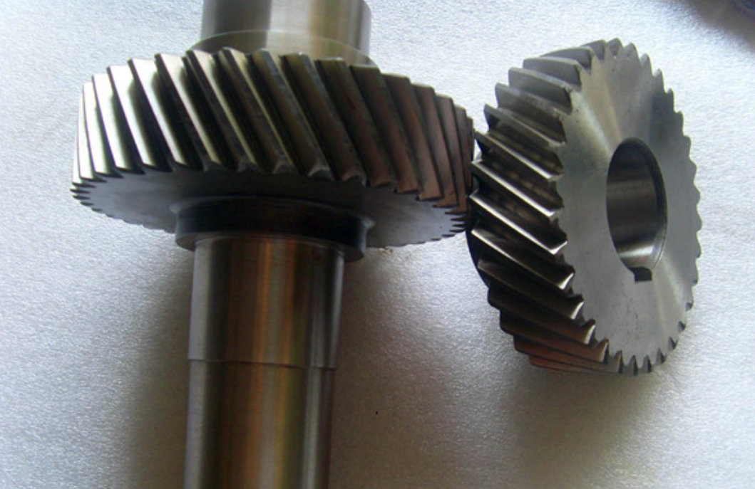
The pursuit of high-performance, low-noise, and highly reliable power transmission systems has placed increasingly stringent demands on the accuracy of gear design and analysis. Central to this endeavor is the creation of a digital twin—a precise three-dimensional model—that faithfully represents the physical gear as it exists after manufacturing, complete with intentional design modifications and unavoidable production deviations. While significant research exists on gear modeling based on the generating principle (simulating a rack or hob tool), the final finishing process for high-precision helical gears is often form grinding. The surface topography resulting from form grinding differs fundamentally from that of generation. Therefore, developing a modeling methodology grounded in the form-machining principle is crucial for achieving simulation models that correlate more accurately with real-world component behavior, especially in finite element analysis (FEA) and dynamic simulations where node equations differ between generation-based and form-based models.
This article presents a comprehensive, step-by-step methodology for constructing a precise digital model of an involute helical gear. The process begins with the derivation of the theoretical tooth profile, proceeds to incorporate common design modifications (profile and lead crowning), and finally integrates key manufacturing errors. All derivations are performed from a first-principles perspective aligned with form-machining concepts.
Theoretical Tooth Profile Foundation
The foundation of any precise gear model is an accurate mathematical description of its tooth flank. For a helical gear, the three-dimensional surface is defined by its transverse (cross-sectional) profile swept along a helical path. We first establish the coordinate system and derive the equations for the transverse profile.
Coordinate System and Involute Curve
A machining coordinate system is established with the gear center as the origin. The y-axis is aligned with the symmetry line of a chosen tooth space. An arbitrary point C on the involute profile is considered. The fundamental geometry of the involute, defined as the trace of a point on a taut string unwinding from a base circle of radius $r_b$, leads to its parametric equations. The transverse pressure angle at an arbitrary radius $r_c$ is $\alpha_c = \arccos(r_b / r_c)$. The involute function is defined as $\text{inv}(\alpha_c) = \tan(\alpha_c) – \alpha_c$.
The coordinates of point C can be expressed in terms of its polar coordinates $(r_c, \theta_c)$: $x = r_c \sin\theta_c$, $y = r_c \cos\theta_c$. The relationship between the tooth thickness at point C, $S_c$, and the standard tooth thickness at the reference circle $S$ is governed by the geometry of the involute. Using the condition of equal arc length in different coordinate representations, the parametric equation for the involute in the machining coordinate system is derived as a function of the local pressure angle $\alpha_c$:
$$
\begin{cases}
x(\alpha_c) = \dfrac{r_b}{\cos(\alpha_c)} \times \sin\left( \dfrac{\pi}{2} + \text{inv}(\alpha) – \text{inv}(\alpha_c) \right) \\[10pt]
y(\alpha_c) = \dfrac{r_b}{\cos(\alpha_c)} \times \cos\left( \dfrac{\pi}{2} + \text{inv}(\alpha) – \text{inv}(\alpha_c) \right)
\end{cases}
$$
Here, $\alpha$ is the standard transverse pressure angle at the reference diameter. This formulation is general and applies to both standard and profile-shifted (modified) helical gears, as the pressure angle $\alpha_c$ is a function of the profile shift coefficient.
Root Fillet Transition Curve
The tooth profile below the start of the active involute (the form diameter) is the root fillet, generated by the tip of the cutting tool. The shape of this fillet depends on the tool geometry. A common tool profile features a double-rounded tip. The key parameters of such a tool are the rack addendum $h_a^* m$, the dedendum $h_f^* m$, the tip radius $r_\rho$, and the tool pressure angle $\alpha_0$. The coordinates $(a, b)$ of the center of the tip rounding relative to the tool datum line are given by:
$$
a = h_f^* m + c^* m – r_\rho, \quad b = \frac{\pi m}{4} + h_f^* m \tan(\alpha_0) + r_\rho \cos(\alpha_0)
$$
where $c^*$ is the clearance coefficient and $m$ is the module. For a full fillet, the tip radius is $r_\rho = c^* m / (1 – \sin \alpha_0)$.
Using the principle of gear generation (tool rack rolling without slippage on the gear’s pitch circle), the root fillet is described as the envelope of the tool tip trochoid. For an arbitrary point D on the fillet, defined by an auxiliary pressure angle $\alpha_D$, the parametric equations in the gear’s coordinate system are:
$$
\begin{cases}
x(\alpha_D) = r \sin \psi – \left( \dfrac{a}{\sin \alpha_D} + r_\rho \right) \cos(\alpha_D – \psi) \\[10pt]
y(\alpha_D) = r \cos \psi – \left( \dfrac{a}{\sin \alpha_D} + r_\rho \right) \sin(\alpha_D – \psi)
\end{cases}
$$
where $r$ is the pitch radius and $\psi = (a / \tan \alpha_D + b) / r$ represents the roll angle. The parameter $\alpha_D$ varies from $\alpha$ (connecting to the involute at the form circle) to $90^\circ$ (connecting to the root circle). For profile-shifted gears, the parameter $a$ is replaced by $a_1 = a \pm x m$, where $x$ is the profile shift coefficient. Combining the equations for the involute segment (valid from the form circle to the tip circle) and the root fillet segment defines the complete theoretical transverse tooth profile.
Incorporating Intentional Modifications
To optimize meshing performance, reduce vibration, and minimize stress concentrations, intentional modifications are applied to the ideal tooth form. The two primary types are profile modification (tip and/or root relief) and lead modification (crowning or end relief).
Profile Modification Modeling
Profile modification involves deliberately altering the involute profile near the tip and/or root. A common strategy is to apply tip relief to the pinion only, or to both mating gears. The modified transverse profile can be divided into four distinct zones, from the tip downwards: the tip relief zone (A-B), the standard involute zone (B-C), the root relief zone (C-D), and the root fillet zone (D-E). The relief amounts $\Delta u_1$ (tip) and $\Delta u_2$ (root) and their corresponding active lengths $g_a$ are determined based on load, deflection, and thermal expansion calculations, often using empirical guidelines.
The relief curve itself can take various forms: parabolic, linear, or circular. We adopt a parabolic form for this discussion. The goal is to define a parabolic segment between points A (at the tip) and B (the start of the true involute) that is tangent to the involute at point B. Let the coordinates of A and B be $(x_A, y_A)$ and $(x_B, y_B)$, respectively. The parabolic curve is defined by $y = ax^2 + bx + c$.
The slope of the involute at point B, $k_B$, is known from its geometry: $k_B = \tan(\alpha_B – \text{inv}(\alpha_B) + \pi/2)$. The slope of the parabola at B is $dy/dx = 2a x_B + b$. Enforcing continuity and tangency at B gives the system of equations to solve for coefficients $a$, $b$, and $c$:
$$
\begin{cases}
y_A = a x_A^2 + b x_A + c \\
y_B = a x_B^2 + b x_B + c \\
k_B = 2a x_B + b
\end{cases}
$$
A similar procedure is applied to model the root relief curve between points C and D, ensuring a smooth transition at point C to the standard involute and at point D to the root fillet. Numerical methods like Gauss-Newton iteration can be used to precisely solve for the transition points ensuring $C^1$ continuity.
Lead (Helix) Modification Modeling
Lead modification alters the tooth profile along its face width to compensate for misalignment and shaft deflection. Common types include end relief (linear or circular chamfer at the ends) and barrel-shaped (crowning) modification. We model a circular end relief. The modification is characterized by the relief amount $\Delta V$ and the active length $g_b$ from each tooth end. When $g_b < b/2$ (where $b$ is face width), it’s end relief; when $g_b = b/2$, it becomes full crowning, but the edge curve remains circular.
For a helical gear, this circular modification in the lead direction manifests as an elliptical arc when projected onto the transverse plane used for our 2D profile. The 3D surface is constructed by sweeping the 2D transverse profile along a helix, while the sweep path itself is modified by this elliptical deviation. The equation of the modifying elliptical path in a plane containing the tooth trace can be defined, and its effect is applied to the basic helix law governing the sweep operation. The composite surface is thus the result of a *modified helical sweep* of the (potentially profile-modified) transverse section.
The table below summarizes common modification strategies for helical gears:
| Modification Type | Typical Form | Primary Purpose | Key Parameters |
|---|---|---|---|
| Profile (Tip/Root Relief) | Parabolic, Linear, Circular | Compensate for bending & shear deflection, reduce mesh-in impact. | Relief amount ($\Delta u$), Relief length ($g_a$). |
| Lead (End Relief) | Circular arc, Linear taper | Compensate for misalignment, prevent edge-loading. | Relief amount ($\Delta V$), Relief length ($g_b$). |
| Lead (Crowning) | Circular arc (barrel-shaped) | Accommodate misalignment and deflection across full face width. | Crown amount ($\Delta V$), usually $g_b = b/2$. |
Integrating Manufacturing Deviations
A truly precise model must account for the inherent inaccuracies of the manufacturing process. The three most critical deviations for gear meshing dynamics are profile deviation, lead deviation, and radial runout (pitch line eccentricity).
Profile and Lead Deviation Mapping
Profile deviation refers to the minute departure of the actual manufactured involute profile from its theoretical (or modified) path. This is typically recorded on a gear inspection chart, which plots error magnitude versus roll length or profile distance. Let us denote the theoretical profile curve (e.g., the involute segment B-C) as $\mathbf{P}_t(\xi) = [X_t(\xi), Y_t(\xi)]$, where $\xi$ is a parameter (e.g., pressure angle $\alpha_c$).
The inspection data provides a deviation function $\delta_p(\ell)$ along the path length $\ell$ of the profile. To apply this to our model, we must map this deviation function onto the theoretical curve. For any point on the theoretical curve corresponding to parameter $\xi$, we calculate the arc length from the start of the evaluated segment:
$$\ell(\xi) = \int_{\xi_0}^{\xi} \sqrt{ \left( \frac{dX_t}{d\xi} \right)^2 + \left( \frac{dY_t}{d\xi} \right)^2 } d\xi$$
The local deviation is $\Delta r(\xi) = \delta_p(\ell(\xi))$. This deviation must be applied in the direction normal to the theoretical profile at that point. The unit normal vector $\hat{n}(\xi)$ at $\mathbf{P}_t(\xi)$ is calculated from the tangent vector. The actual profile point is then:
$$\mathbf{P}_a(\xi) = \mathbf{P}_t(\xi) + \Delta r(\xi) \cdot \hat{n}(\xi)$$
The deviation function $\delta_p(\ell)$ is often obtained by fitting a curve to discrete inspection data. For example, an inspection plot might be digitized and fitted with a function combining harmonic and polynomial terms, such as:
$$\delta_p(\ell) = a \sin(\omega \ell – \phi) + b (\ell – \ell_0)^n + c$$
Coefficients $a, b, c, \omega, \phi, n, \ell_0$ are determined via non-linear least-squares fitting (e.g., minimizing residual sum of squares), and the fit quality can be assessed using metrics like Normalized Root Mean Square Error (NRMSE). An identical methodology is applied to map lead deviation data, $\delta_l(z)$, along the face width $z$, onto the helical lead of the tooth flank.
Radial Runout (Eccentricity) Integration
Radial runout, often due to mounting eccentricity, causes a periodic variation in the radial position of successive teeth. This is measured as the total indicator reading (TIR) as the gear rotates. The runout error is typically plotted as a function of angular position $\theta$. This error $\delta_r(\theta)$ represents the radial displacement of the theoretical pitch circle.
To model this, we first construct the gear model with one “perfect” tooth in its nominal position. The runout function $\delta_r(\theta)$ is used to create a modified polar array pattern. Instead of placing each tooth at a constant radius $r$ and evenly spaced angles $2\pi i / Z$ (for $i=0$ to $Z-1$, where $Z$ is the number of teeth), the $i$-th tooth is placed at a radius $r + \delta_r(2\pi i / Z)$ and at its nominal angular position. This effectively distorts the tooth-to-tooth spacing and the true operating pitch circle, replicating the effect of eccentricity. A Fourier series is often suitable for fitting the periodic runout data:
$$\delta_r(\theta) = \sum_{k=1}^{N} [A_k \cos(k\theta) + B_k \sin(k\theta)]$$
The complete modeling workflow, synthesizing all derived equations for the theoretical form, modifications, and deviations, is summarized in the following table:
| Modeling Stage | Mathematical Description | Key Inputs/Parameters | Output |
|---|---|---|---|
| 1. Theoretical Profile | Eqns. (1) for involute, Eqns. (2) for root fillet. $\alpha_c$ or $\alpha_D$ as parameter. | $m, Z, \alpha, \beta, x, h_a^*, c^*, r_\rho$. | Perfect transverse 2D profile. |
| 2. Profile Modification | Parabolic curves (Eqns. 3) attached to involute ends. | $\Delta u_1, \Delta u_2, g_a$, modification type. | Modified 2D profile. |
| 3. Lead Modification | Modified helical sweep with elliptical/circular path (Eqns. 4 implied in sweep law). | $\Delta V, g_b$, face width $b$, helix angle $\beta$. | Modified 3D tooth surface. |
| 4. Profile/Lead Deviation | $\mathbf{P}_a(\xi) = \mathbf{P}_t(\xi) + \delta_{p,l}(\ell) \cdot \hat{n}(\xi)$. | Fitted deviation functions $\delta_p(\ell)$, $\delta_l(z)$ from inspection data. | 3D surface with micro-geometry errors. |
| 5. Radial Runout | Tooth positioning: $r_i = r + \delta_r(2\pi i / Z)$. | Fitted runout function $\delta_r(\theta)$ from inspection. | Complete gear model with eccentricity. |
Synthesis and Model Generation
The final model is generated through a procedural algorithm that implements the stages above. A parameterized script is written, which accepts basic gear geometry, modification parameters, and data arrays for the fitted deviation functions. The process begins by generating the sequence of curves for a single transverse tooth profile: tip relief parabola, main involute, root relief parabola, and root fillet trochoid. Numerical methods ensure $C^1$ continuity at junctions B, C, and D.
This 2D profile is then swept along a helical path to create a 3D surface. The lead modification is integrated by modulating the sweep path according to its defined law (e.g., an elliptical arc). The profile and lead deviation functions are then evaluated and used to perturb the vertices or control points of this 3D surface along their local normals, imprinting the measured micro-geometry.
This results in a precise model for a single tooth. Finally, the radial runout function is evaluated at each tooth index position $i$. A transformation matrix for each tooth is computed, combining the nominal rotation $(2\pi i / Z)$ with a radial translation of magnitude $\delta_r(2\pi i / Z)$. The single-tooth model is instanced using these varying transformation matrices to create the full gear assembly. This gear model accurately reflects the intended design modifications and the measured signature of manufacturing process variations.
Conclusion
This article has detailed a first-principles methodology for constructing a high-fidelity digital model of a helical gear. The approach is firmly rooted in the form-machining principle, which underlies common finishing processes like form grinding. Starting from the fundamental equations of the involute and root fillet, the method systematically incorporates the mathematical definitions of profile and lead modifications. Crucially, it demonstrates a procedural framework for integrating real-world manufacturing deviations—profile error, lead error, and radial runout—by mapping fitted inspection data onto the nominal tooth flank geometry. The final output is a comprehensive 3D solid model that serves as a true digital twin of the physical component. Such precise models are indispensable for advanced computational analyses, including non-linear contact FEA and system-level dynamic simulation, where the accurate representation of micro-geometry and imperfections is essential for predicting vibration, noise, stress distribution, and fatigue life with high confidence. The ability to generate these models forms the critical link between design intent, manufacturing reality, and predictive performance engineering for helical gears.