
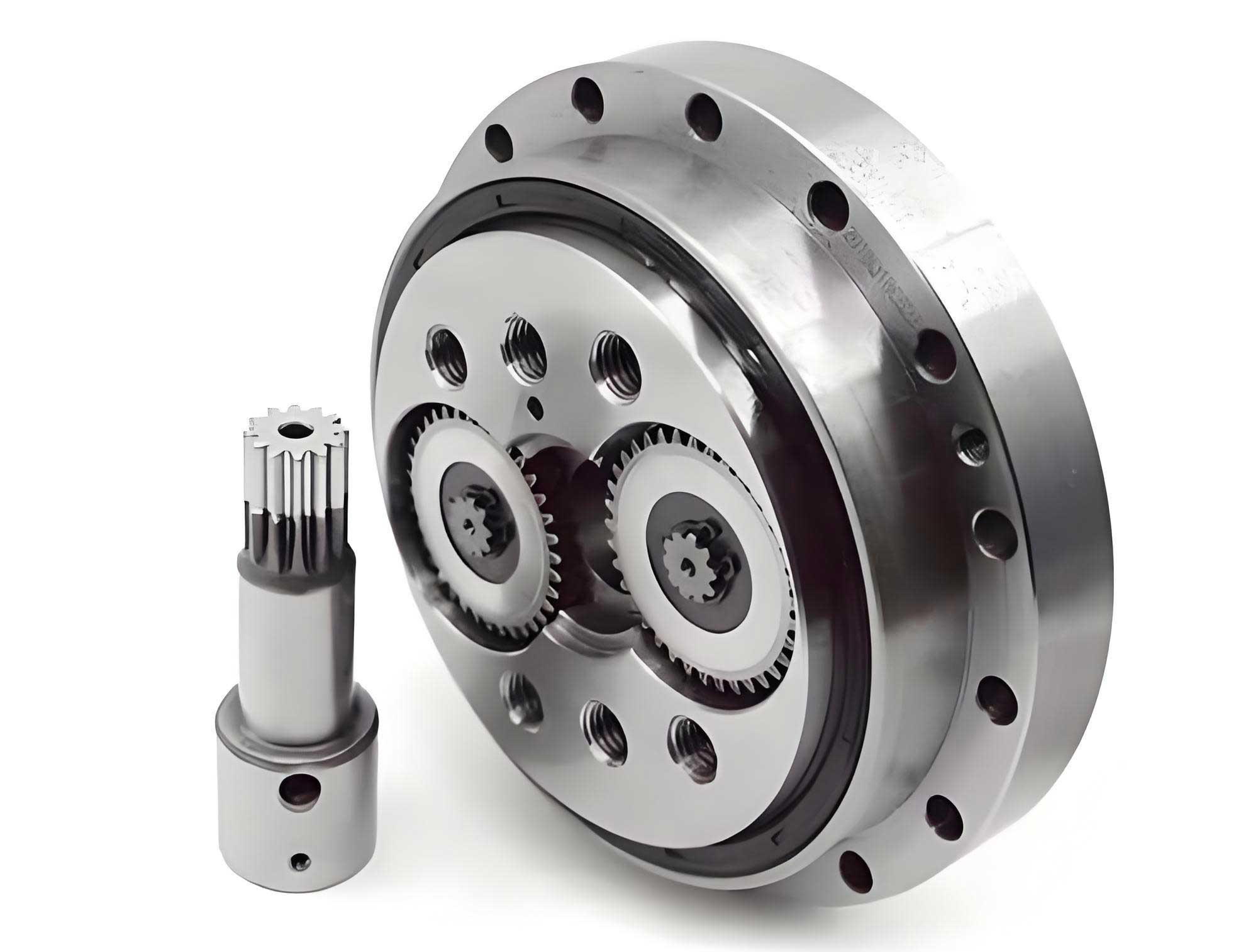
In the field of high-precision industrial robotics, the rotary vector reducer plays a critical role due to its compact design, high torque capacity, and exceptional accuracy. As a researcher focused on advanced manufacturing systems, I have extensively studied the grinding processes for cycloid wheels, which are core components of rotary vector reducers. The final machining step—form grinding—directly determines the齿廓精度 of the cycloid wheel, with stringent requirements: dimensional errors within ±2 μm, surface roughness below Ra 0.4, and indexing errors between teeth within one arc-minute. Achieving such precision necessitates a deep understanding of the grinding machine’s motion errors, as even minor deviations in the machine tool’s geometric and kinematic parameters can lead to significant quality degradation. This article presents a comprehensive error analysis and modeling approach for the grinding system of a CNC cycloid wheel grinder, based on multi-body system theory. I will derive a universal spatial error model, establish precision grinding constraints, and demonstrate how to predict machining accuracy, all while emphasizing the importance of the rotary vector reducer in modern automation.
The foundation of this work lies in multi-body system theory, which simplifies complex mechanical systems by decomposing them into interconnected rigid bodies. From my perspective, this approach allows for systematic error propagation analysis. Consider two adjacent bodies, B_i and B_j, where B_i is the lower-order body. In an ideal, error-free scenario, the relative position and orientation between them can be described using coordinate systems attached to each body. Let O_i – x_i y_i z_i and O_j – x_j y_j z_j denote the body-fixed coordinate systems for B_i and B_j, respectively. The relative positioning is represented by a vector q_j from O_i to a reference point Q_j on B_j, and the relative motion is described by a displacement vector s_j from Q_j to O_j. For any point P on B_j, its position vector in the O_i – x_i y_i z_i coordinate system is given by:
$$ \mathbf{P} = \mathbf{q}_j + \mathbf{s}_j + \mathbf{r}_j $$
where \(\mathbf{r}_j\) is the position vector of point P in the O_j – x_j y_j z_j system. This can be expressed using Denavit-Hartenberg (D-H) homogeneous transformation matrices. Let \( \mathbf{P}_j^i \) be the homogeneous coordinate matrix of point P in the O_i – x_i y_i z_i system, and \( \mathbf{S}_j^r \) be its matrix in the O_j – x_j y_j z_j system. The transformation is:
$$ \mathbf{P}_j^i = \mathbf{S}_{ij}^p \mathbf{S}_{ij}^s \mathbf{S}_j^r $$
Here, \( \mathbf{S}_{ij}^p \) is the relative positioning transformation matrix from B_i to B_j, and \( \mathbf{S}_{ij}^s \) is the relative motion transformation matrix. However, in real-world grinding systems for rotary vector reducers, errors are inevitable. These include geometric errors such as straightness, squareness, and angular deviations, as well as motion-dependent errors like positional inaccuracies. To model this, I introduce error vectors. Let \( \mathbf{q}_{jl} \) and \( \mathbf{s}_{jl} \) be the ideal positioning and displacement vectors, respectively, while \( \mathbf{q}_{je} \) and \( \mathbf{s}_{je} \) represent the corresponding error vectors. Thus, the actual position vector becomes:
$$ \mathbf{P} = \mathbf{q}_{jl} + \mathbf{q}_{je} + \mathbf{s}_{jl} + \mathbf{s}_{je} + \mathbf{r}_j $$
In matrix form, this extends to:
$$ \mathbf{P}_j^i = \mathbf{S}_{ij}^p \mathbf{S}_{ij}^{pe} \mathbf{S}_{ij}^s \mathbf{S}_{ij}^{se} \mathbf{S}_j^r $$
where \( \mathbf{S}_{ij}^{pe} \) and \( \mathbf{S}_{ij}^{se} \) are the error transformation matrices for positioning and motion, respectively. This formulation is crucial for capturing the nuanced errors in a rotary vector reducer’s grinding process, as it accounts for both static and dynamic inaccuracies.
To apply this theory, I analyze a specific CNC cycloid wheel grinding machine, similar to the LFG-3540 model. This machine is a four-axis system utilizing form grinding, where the grinding wheel rotates, the Z-axis moves the cycloid wheel laterally, the Y-axis controls the depth of cut, the X-axis adjusts the grinding wheel head vertically, and the A-axis provides indexing. Each axis contributes geometric errors that affect the final wheel profile. From my investigation, these errors can be categorized into static (position-independent) and dynamic (position-dependent) errors. Static errors include squareness errors between axes, such as \( \varepsilon_{xy} \), \( \varepsilon_{xz} \), and \( \varepsilon_{yz} \) between the linear axes, and \( \varepsilon_{xa} \), \( \varepsilon_{ya} \) between the linear axes and the rotary A-axis. Dynamic errors arise from guideway imperfections and thermal effects, resulting in six error components per axis: three linear displacement errors and three angular errors. For instance, as the X-axis moves, it exhibits errors \( \delta_x(x) \), \( \delta_y(x) \), \( \delta_z(x) \) in linear displacements and \( \varepsilon_x(x) \), \( \varepsilon_y(x) \), \( \varepsilon_z(x) \) in angular rotations. Similarly, other axes have analogous error parameters. To summarize, I list all geometric error parameters in the following table, which is essential for modeling the grinding system of a rotary vector reducer component.
| Error Type | Linear Displacement Errors | Angular Displacement Errors | Direction |
|---|---|---|---|
| Along X translation | \( \delta_x(x) \), \( \delta_y(x) \), \( \delta_z(x) \) | \( \varepsilon_x(x) \), \( \varepsilon_y(x) \), \( \varepsilon_z(x) \) | Along x, y, z |
| Along Y translation | \( \delta_x(y) \), \( \delta_y(y) \), \( \delta_z(y) \) | \( \varepsilon_x(y) \), \( \varepsilon_y(y) \), \( \varepsilon_z(y) \) | Along x, y, z |
| Along Z translation | \( \delta_x(z) \), \( \delta_y(z) \), \( \delta_z(z) \) | \( \varepsilon_x(z) \), \( \varepsilon_y(z) \), \( \varepsilon_z(z) \) | Along x, y, z |
| Around A rotation | \( \delta_x(a) \), \( \delta_y(a) \), \( \delta_z(a) \) | \( \varepsilon_x(a) \), \( \varepsilon_y(a) \), \( \varepsilon_z(a) \) | Around x, y, z |
| Cross-axis squareness | \( \varepsilon_{xy} \), \( \varepsilon_{xz} \), \( \varepsilon_{yz} \), \( \varepsilon_{xa} \), \( \varepsilon_{ya} \) | ||
This comprehensive error set forms the basis for the multi-body system model. Next, I abstract the grinding system into a multi-body topology. The machine consists of two main kinematic chains: the “bed-cycloid wheel” branch (bed → Z-slide → headstock → A-axis → cycloid wheel) and the “bed-grinding wheel” branch (bed → Y-slide → X-slide → wheel head → grinding wheel). Using low-order body array notation, where \( L^n(j) = i \) indicates that body B_i is the n-th order lower body of B_j, I derive the topological relationships. Let k represent the body index: 1 for bed, 2 for Z-slide, 3 for headstock, 4 for A-axis, 5 for cycloid wheel, 6 for Y-slide, 7 for X-slide, 8 for wheel head, and 9 for grinding wheel. The low-order body array is computed as follows:
| k | 1 | 2 | 3 | 4 | 5 | 6 | 7 | 8 | 9 |
|---|---|---|---|---|---|---|---|---|---|
| L1(k) | 0 | 1 | 2 | 3 | 4 | 1 | 6 | 7 | 8 |
| L2(k) | 0 | 0 | 1 | 2 | 3 | 0 | 1 | 6 | 7 |
| L3(k) | 0 | 0 | 0 | 1 | 2 | 0 | 0 | 1 | 6 |
| L4(k) | 0 | 0 | 0 | 0 | 1 | 0 | 0 | 0 | 1 |
| L5(k) | 0 | 0 | 0 | 0 | 0 | 0 | 0 | 0 | 0 |
This array succinctly captures the hierarchical structure, facilitating the error modeling. With the topology defined, I proceed to establish coordinate systems for each body. The inertial coordinate system is fixed to the bed (body 1). For the “bed-cycloid wheel” branch, I align the coordinate systems of the Z-slide (body 2) and headstock (body 3) with the bed system, as they are rigidly connected. The A-axis (body 4) coordinate system is oriented by rotating the bed system by squareness errors \( \varepsilon_{xa} \) and \( \varepsilon_{ya} \). The cycloid wheel (body 5) system shares the orientation of the A-axis. For the “bed-grinding wheel” branch, the Y-slide (body 6) system aligns with the bed, while the X-slide (body 7) system is oriented by rotating for squareness errors \( \varepsilon_{xy} \), \( \varepsilon_{xz} \), and \( \varepsilon_{yz} \). The wheel head (body 8) and grinding wheel (body 9) systems match the X-slide orientation. Positionally, I set the origins of bodies 1-4 and 6-8 at the A-axis center in the initial machine zero position, with the cycloid wheel and grinding wheel origins at their respective body centers. Let \( \mathbf{q}_5 = [q_{5x}, q_{5y}, q_{5z}, 1]^T \) be the position of the cycloid wheel system relative to the A-axis, and \( \mathbf{S}_{5r} = [x_w, y_w, z_w, 1]^T \) be the point P on the cycloid wheel in its local system. Similarly, for the grinding wheel, \( \mathbf{q}_9 = [q_{9x}, q_{9y}, q_{9z}, 1]^T \) and \( \mathbf{S}_{9r} = [x_t, y_t, z_t, 1]^T \).
Now, I derive the D-H transformation matrices for each adjacent pair in both branches. For the “bed-cycloid wheel” branch, the matrices are as follows. Between bed (1) and Z-slide (2): \( \mathbf{S}_{12}^p = \mathbf{I} \) (identity for ideal positioning), \( \mathbf{S}_{12}^{pe} = \mathbf{I} \) (no positioning error initially), \( \mathbf{S}_{12}^s = \begin{bmatrix} 1 & 0 & 0 & 0 \\ 0 & 1 & 0 & 0 \\ 0 & 0 & 1 & z \\ 0 & 0 & 0 & 1 \end{bmatrix} \) for Z-motion, and \( \mathbf{S}_{12}^{se} = \begin{bmatrix} 1 & -\varepsilon_z(z) & \varepsilon_y(z) & \delta_x(z) \\ \varepsilon_z(z) & 1 & -\varepsilon_x(z) & \delta_y(z) \\ -\varepsilon_y(z) & \varepsilon_x(z) & 1 & \delta_z(z) \\ 0 & 0 & 0 & 1 \end{bmatrix} \) for Z-axis motion errors. Between Z-slide (2) and headstock (3): all matrices are identity since they are fixed. Between headstock (3) and A-axis (4): \( \mathbf{S}_{34}^p = \mathbf{I} \), \( \mathbf{S}_{34}^{pe} = \begin{bmatrix} 1 & 0 & \varepsilon_{xa} & 0 \\ 0 & 1 & -\varepsilon_{ya} & 0 \\ -\varepsilon_{xa} & \varepsilon_{ya} & 1 & 0 \\ 0 & 0 & 0 & 1 \end{bmatrix} \), \( \mathbf{S}_{34}^s = \begin{bmatrix} \cos\alpha & -\sin\alpha & 0 & 0 \\ \sin\alpha & \cos\alpha & 0 & 0 \\ 0 & 0 & 1 & 0 \\ 0 & 0 & 0 & 1 \end{bmatrix} \) for A-rotation by angle \( \alpha \), and \( \mathbf{S}_{34}^{se} = \begin{bmatrix} 1 & -\varepsilon_z(a) & \varepsilon_y(a) & \delta_x(a) \\ \varepsilon_z(a) & 1 & -\varepsilon_x(a) & \delta_y(a) \\ -\varepsilon_y(a) & \varepsilon_x(a) & 1 & \delta_z(a) \\ 0 & 0 & 0 & 1 \end{bmatrix} \). Between A-axis (4) and cycloid wheel (5): \( \mathbf{S}_{45}^p = \begin{bmatrix} 1 & 0 & 0 & q_{5x} \\ 0 & 1 & 0 & q_{5y} \\ 0 & 0 & 1 & q_{5z} \\ 0 & 0 & 0 & 1 \end{bmatrix} \), with error matrices as identity. For the “bed-grinding wheel” branch, similar matrices are defined. Between bed (1) and Y-slide (6): \( \mathbf{S}_{16}^p = \mathbf{I} \), \( \mathbf{S}_{16}^{pe} = \mathbf{I} \), \( \mathbf{S}_{16}^s = \begin{bmatrix} 1 & 0 & 0 & 0 \\ 0 & 1 & 0 & y \\ 0 & 0 & 1 & 0 \\ 0 & 0 & 0 & 1 \end{bmatrix} \), and \( \mathbf{S}_{16}^{se} = \begin{bmatrix} 1 & -\varepsilon_z(y) & \varepsilon_y(y) & \delta_x(y) \\ \varepsilon_z(y) & 1 & -\varepsilon_x(y) & \delta_y(y) \\ -\varepsilon_y(y) & \varepsilon_x(y) & 1 & \delta_z(y) \\ 0 & 0 & 0 & 1 \end{bmatrix} \). Between Y-slide (6) and X-slide (7): \( \mathbf{S}_{67}^p = \mathbf{I} \), \( \mathbf{S}_{67}^{pe} = \begin{bmatrix} 1 & -\varepsilon_{xy} & \varepsilon_{xz} & 0 \\ \varepsilon_{xy} & 1 & -\varepsilon_{yz} & 0 \\ -\varepsilon_{xz} & \varepsilon_{yz} & 1 & 0 \\ 0 & 0 & 0 & 1 \end{bmatrix} \), \( \mathbf{S}_{67}^s = \begin{bmatrix} 1 & 0 & 0 & x \\ 0 & 1 & 0 & 0 \\ 0 & 0 & 1 & 0 \\ 0 & 0 & 0 & 1 \end{bmatrix} \), and \( \mathbf{S}_{67}^{se} = \begin{bmatrix} 1 & -\varepsilon_z(x) & \varepsilon_y(x) & \delta_x(x) \\ \varepsilon_z(x) & 1 & -\varepsilon_x(x) & \delta_y(x) \\ -\varepsilon_y(x) & \varepsilon_x(x) & 1 & \delta_z(x) \\ 0 & 0 & 0 & 1 \end{bmatrix} \). Between X-slide (7) and wheel head (8): identity matrices. Between wheel head (8) and grinding wheel (9): \( \mathbf{S}_{89}^p = \begin{bmatrix} 1 & 0 & 0 & q_{9x} \\ 0 & 1 & 0 & q_{9y} \\ 0 & 0 & 1 & q_{9z} \\ 0 & 0 & 0 & 1 \end{bmatrix} \), with error matrices as identity.
Using these matrices, I compute the position of point P—the grinding contact point—in the inertial coordinate system via both branches. For the “bed-cycloid wheel” branch, the total transformation is:
$$ \mathbf{P}_w = \mathbf{S}_{12}^p \mathbf{S}_{12}^{pe} \mathbf{S}_{12}^s \mathbf{S}_{12}^{se} \mathbf{S}_{23}^p \mathbf{S}_{23}^{pe} \mathbf{S}_{23}^s \mathbf{S}_{23}^{se} \mathbf{S}_{34}^p \mathbf{S}_{34}^{pe} \mathbf{S}_{34}^s \mathbf{S}_{34}^{se} \mathbf{S}_{45}^p \mathbf{S}_{45}^{pe} \mathbf{S}_{45}^s \mathbf{S}_{45}^{se} \mathbf{S}_{5r} $$
For the “bed-grinding wheel” branch:
$$ \mathbf{P}_t = \mathbf{S}_{16}^p \mathbf{S}_{16}^{pe} \mathbf{S}_{16}^s \mathbf{S}_{16}^{se} \mathbf{S}_{67}^p \mathbf{S}_{67}^{pe} \mathbf{S}_{67}^s \mathbf{S}_{67}^{se} \mathbf{S}_{78}^p \mathbf{S}_{78}^{pe} \mathbf{S}_{78}^s \mathbf{S}_{78}^{se} \mathbf{S}_{89}^p \mathbf{S}_{89}^{pe} \mathbf{S}_{89}^s \mathbf{S}_{89}^{se} \mathbf{S}_{9r} $$
Performing the matrix multiplications symbolically, I obtain the expressions for \( \mathbf{P}_w = [x_{w0}, y_{w0}, z_{w0}, 1]^T \) and \( \mathbf{P}_t = [x_{t0}, y_{t0}, z_{t0}, 1]^T \). For brevity, I summarize the results. The cycloid wheel branch yields:
$$ x_{w0} = \delta_x(a) \cos\alpha – \delta_y(a) \sin\alpha + \delta_x(z) + (x_w + q_{5x})[\cos\alpha – \varepsilon_z(z) \sin\alpha – \varepsilon_z(a) \sin\alpha] – (y_w + q_{5y})[\sin\alpha + \varepsilon_z(z) \cos\alpha + \varepsilon_z(a) \cos\alpha] + (z_w + q_{5z})[\varepsilon_{xa} + \varepsilon_y(z) + \sin\alpha + \varepsilon_x(a) \sin\alpha + \varepsilon_y(a) \cos\alpha] $$
$$ y_{w0} = \delta_x(a) \sin\alpha + \delta_y(a) \cos\alpha + \delta_y(z) + (x_w + q_{5x})[\cos\alpha + \sin\alpha + \varepsilon_z(a) \cos\alpha] + (y_w + q_{5y})[\cos\alpha – \varepsilon_z(z) \sin\alpha – \varepsilon_z(a) \sin\alpha] – (z_w + q_{5z})[\varepsilon_{ya} + \varepsilon_x(z) + \sin\alpha + \varepsilon_x(a) \cos\alpha – \varepsilon_y(a) \sin\alpha] $$
$$ z_{w0} = z + \delta_z(a) + \delta_z(z) – (x_w + q_{5x})\{ \varepsilon_y(a) + \cos\alpha[\varepsilon_{xa} + \varepsilon_y(z)] – \sin\alpha[\varepsilon_{ya} + \varepsilon_x(z)] \} + (y_w + q_{5y})\{ \varepsilon_x(a) + \cos\alpha[\varepsilon_{ya} + \varepsilon_x(z)] + \sin\alpha[\varepsilon_{xa} + \varepsilon_y(z)] \} + z_w + q_{5z} $$
The grinding wheel branch gives:
$$ x_{t0} = x + \delta_x(x) + \delta_x(y) + x_t + q_{9x} – (y_t + q_{9y})[\varepsilon_{xy} + \varepsilon_z(x) + \varepsilon_z(y)] + (z_t + q_{9z})[\varepsilon_{xz} + \varepsilon_y(x) + \varepsilon_y(y)] $$
$$ y_{t0} = x[\varepsilon_{xy} + \varepsilon_z(y)] + y + \delta_y(x) + \delta_y(y) + (x_t + q_{9x})[\varepsilon_z(x) + \varepsilon_z(y) + \varepsilon_{xy}] + y_t + q_{9y} – (z_t + q_{9z})[\delta_y(x) + \delta_y(y) + x(\varepsilon_{xy} + \varepsilon_z(y)) + y] $$
$$ z_{t0} = \delta_z(x) + \delta_z(y) – x[\varepsilon_{xz} + \varepsilon_y(y)] – (x_t + q_{9x})[\varepsilon_y(x) + \varepsilon_y(y) + \varepsilon_{xz}] + (y_t + q_{9y})[\varepsilon_{yz} + \varepsilon_x(x) + \varepsilon_x(y)] + z_t + q_{9z} $$
Precision grinding of the rotary vector reducer’s cycloid wheel requires that the grinding point on the wheel coincides with the theoretical point on the cycloid wheel at all times. Thus, the constraint equation is \( \mathbf{P}_w = \mathbf{P}_t \). Setting the corresponding components equal, I derive the precision grinding constraint equation as a system of three equations. For the x-component:
$$ \delta_x(a) \cos\alpha – \delta_y(a) \sin\alpha + \delta_x(z) + (x_w + q_{5x})[\cos\alpha – \varepsilon_z(z) \sin\alpha – \varepsilon_z(a) \sin\alpha] – (y_w + q_{5y})[\sin\alpha + \varepsilon_z(z) \cos\alpha + \varepsilon_z(a) \cos\alpha] + (z_w + q_{5z})[\varepsilon_{xa} + \varepsilon_y(z) + \sin\alpha + \varepsilon_x(a) \sin\alpha + \varepsilon_y(a) \cos\alpha] = x + \delta_x(x) + \delta_x(y) + x_t + q_{9x} – (y_t + q_{9y})[\varepsilon_{xy} + \varepsilon_z(x) + \varepsilon_z(y)] + (z_t + q_{9z})[\varepsilon_{xz} + \varepsilon_y(x) + \varepsilon_y(y)] $$
For the y-component:
$$ \delta_x(a) \sin\alpha + \delta_y(a) \cos\alpha + \delta_y(z) + (x_w + q_{5x})[\cos\alpha + sin\alpha + \varepsilon_z(a) \cos\alpha] + (y_w + q_{5y})[\cos\alpha – \varepsilon_z(z) \sin\alpha – \varepsilon_z(a) \sin\alpha] – (z_w + q_{5z})[\varepsilon_{ya} + \varepsilon_x(z) + sin\alpha + \varepsilon_x(a) \cos\alpha – \varepsilon_y(a) \sin\alpha] = x[\varepsilon_{xy} + \varepsilon_z(y)] + y + \delta_y(x) + \delta_y(y) + (x_t + q_{9x})[\varepsilon_z(x) + \varepsilon_z(y) + \varepsilon_{xy}] + y_t + q_{9y} – (z_t + q_{9z})[\delta_y(x) + \delta_y(y) + x(\varepsilon_{xy} + \varepsilon_z(y)) + y] $$
For the z-component:
$$ z + \delta_z(a) + \delta_z(z) – (x_w + q_{5x})\{ \varepsilon_y(a) + \cos\alpha[\varepsilon_{xa} + \varepsilon_y(z)] – \sin\alpha[\varepsilon_{ya} + \varepsilon_x(z)] \} + (y_w + q_{5y})\{ \varepsilon_x(a) + \cos\alpha[\varepsilon_{ya} + \varepsilon_x(z)] + \sin\alpha[\varepsilon_{xa} + \varepsilon_y(z)] \} + z_w + q_{5z} = \delta_z(x) + \delta_z(y) – x[\varepsilon_{xz} + \varepsilon_y(y)] – (x_t + q_{9x})[\varepsilon_y(x) + \varepsilon_y(y) + \varepsilon_{xz}] + (y_t + q_{9y})[\varepsilon_{yz} + \varepsilon_x(x) + \varepsilon_x(y)] + z_t + q_{9z} $$
This system encapsulates all 29 geometric error parameters listed earlier. In practice, to predict the machining accuracy for a rotary vector reducer’s cycloid wheel, one can measure or estimate these error parameters using standard geometric calibration techniques, such as laser interferometry or ball-bar tests, as per specifications like JB/T 8772.1-1998. By substituting the error values into the constraint equation and evaluating the residual \( \mathbf{E} = \mathbf{P}_w – \mathbf{P}_t \), the deviation from ideal grinding conditions can be quantified. This enables proactive error compensation or machine adjustment to ensure the high precision required for rotary vector reducers.
From my analysis, several insights emerge. First, the multi-body system approach provides a structured framework for error modeling, adaptable to various machine configurations. Second, the constraint equation highlights the complex interplay between linear and rotary axes errors, emphasizing the need for comprehensive calibration in rotary vector reducer manufacturing. Third, by incorporating error matrices into the D-H transformations, the model accounts for both systematic and random errors, enhancing its predictive capability. I have also considered extensions, such as thermal errors or dynamic effects, which could be integrated by adding relevant error terms to the matrices. Moreover, this model can serve as a foundation for real-time error compensation systems in CNC grinders, potentially improving the consistency and quality of rotary vector reducer components.
In conclusion, this study presents a detailed error analysis and modeling methodology for the grinding system of a cycloid wheel used in rotary vector reducers. By leveraging multi-body system theory, I have derived a universal spatial error model that captures 29 geometric error parameters through D-H transformation matrices. The precision grinding constraint equation, derived from equating the grinding point positions along two kinematic branches, provides a direct means to assess machining accuracy. This work not only advances the understanding of error propagation in precision grinding but also offers practical tools for machine tool calibration and optimization. Future research could focus on experimental validation, integration with sensor data for adaptive control, and extension to other complex machining processes for rotary vector reducers. As the demand for high-performance robotics grows, such precision engineering approaches will remain vital for advancing rotary vector reducer technology and ensuring the reliability of industrial automation systems.