
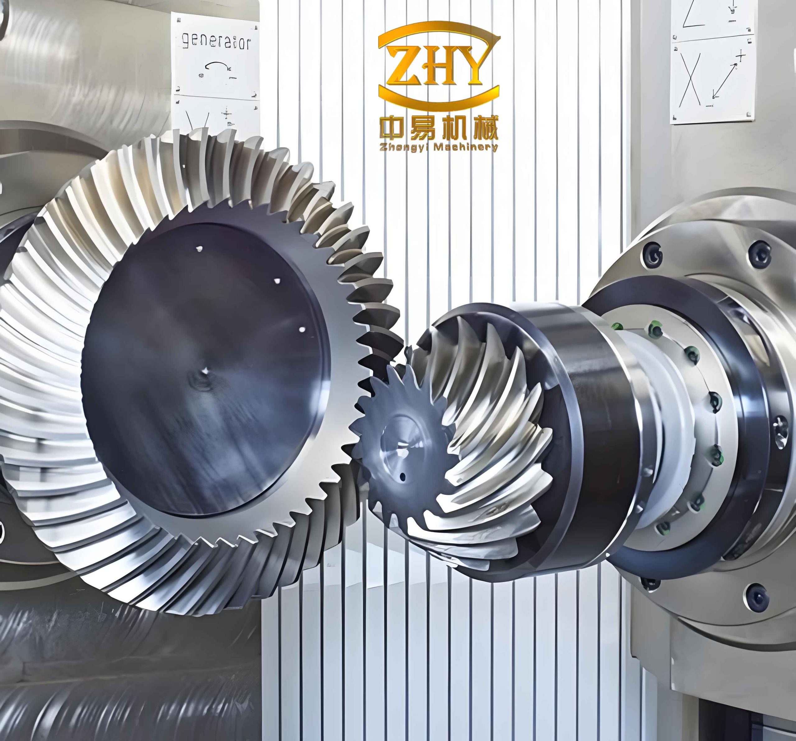
The precise manufacturing of hyperboloid gears, specifically hypoid gears, represents a significant challenge in advanced gear technology. Unlike conventional gears, the complex, spatially curved tooth flanks of hypoid gears cannot be generated by simple hobbling or shaping processes. Instead, they are produced on specialized machine tools, such as Gleason machines or modern CNC hypoid generators, where the cutter and workpiece undergo a complex series of coordinated motions. The quality of the final gear mesh—characterized by contact pattern area, position, and transmission error—is critically dependent on the accurate setting of numerous machine tool parameters. Even minor deviations in these settings can lead to poor contact, high stress concentration, noise, and reduced load capacity. Traditional manufacturing relies heavily on iterative trial-and-error adjustments, involving repeated cutting, assembly, and contact pattern testing with a mating gear. This process is not only time-consuming and costly but also limits the interchangeability of manufactured gears. This article presents a method to fundamentally improve this paradigm by using three-dimensional coordinate measurement data from a finished gear tooth surface to directly recover the actual machining parameters used during its production. This reverse-engineering approach allows for the precise replication of successful gear geometry and offers a path toward achieving functional interchangeability for hyperboloid gears.
The core of this method lies in establishing a rigorous mathematical link between the machine tool’s kinematic configuration and the resulting tooth surface geometry. For a hypoid pinion (often referred to as the “angular gear” in a hypoid set), the surface is generated by the envelope of a cutting tool (like a single-point cutter) as it moves relative to the gear blank according to the machine’s setup. The mathematical model describes the tooth surface as a function of the tool geometry and a set of machine adjustment parameters. Let us define the coordinate systems. The machine tool coordinate system is denoted as $O-VHZ$. The angular gear coordinate system is $O_p-x_p y_p z_p$, with its origin $O_p$ at the apex of the gear’s pitch cone and the $y_p$-axis coinciding with the gear axis. At the initial rotational position, the $x_p$-axis is parallel to the machine’s $V$-axis.
The cutter center in the machine coordinate system is represented by the vector $\mathbf{D}_p(V_p, H_p, -Z_p)$. The components defining its orientation and the parameters $V_p$, $H_p$ are governed by the machine’s adjustment angles $\phi_1, \phi_2, \phi_3, \phi_4$ and other constants like the machine eccentricity $E_x$ and the cutter blade angle $\gamma$. The relationships are given by a series of trigonometric functions. For instance, a key orientation component $a_{pz}$ and the derived $V_p$, $H_p$ can be expressed as:
$$
a_{pz} = \cos \varphi_1 \sin \gamma + \cos \gamma \sqrt{1 – \cos^2 \varphi_1 \sin^2 \gamma}
$$
Depending on the quadrant of $\varphi_1$, the calculations for $H_p$ and $V_p$ follow specific branches, such as:
$$
H_p = E_x \tan \varphi_2, \quad V_p = H_p / \tan \varphi_1 \quad \text{for} \quad \theta_1 < \varphi_1 < \theta_2
$$
where $\theta_1$ and $\theta_2$ are boundary angles defined based on $\varphi_3$ and $\varphi_4$.
As the cutter rotates about its axis with an angular parameter $\varphi$ and the gear blank rotates with a ratio $i\varphi$, the cutting edge sweeps out the tooth surface. The locus of a point $\mathbf{X}_{pc}$ on the cutting edge, transformed into the machine coordinate system, is:
$$
\mathbf{X}_{p\varphi}(u_p, v_p; \varphi) = \mathbf{C}(\varphi)\mathbf{B}(\beta)\mathbf{A}(\alpha)[\mathbf{X}_{pc}(u_p, v_p)] + \mathbf{D}_p
$$
Here, $u_p$ and $v_p$ are parameters defining a point on the cutter blade, and $\mathbf{A}(\alpha)$, $\mathbf{B}(\beta)$, $\mathbf{C}(\varphi)$ are transformation matrices for rotations about different axes. The condition for the surface being the envelope of the family of cutter positions is that the relative velocity between the cutter and the workpiece is orthogonal to the surface normal at the point of contact. This is expressed by the equation:
$$
\mathbf{N}_{p\varphi} \cdot \mathbf{W} = 0
$$
where $\mathbf{N}_{p\varphi}$ is the unit normal vector to the cutter surface at the point in question, and $\mathbf{W}$ is the relative velocity vector, calculated from the velocities of the cutter point and the corresponding point on the gear. Solving this equation allows us to express one of the surface parameters, say $v_p$, as a function of the other and the motion parameter: $v_p = v_p(u_p; \varphi)$. Substituting this back gives the equation of the cutting line $L$ for a fixed $\varphi$, and the final tooth surface of the hyperboloid angular gear in its own coordinate system is:
$$
\mathbf{X}_p(u_p; \varphi) = \mathbf{B}^{-1}(\lambda_p)\mathbf{A}^{-1}(i\varphi)[L(u_p; \varphi) – (0, 0, Y_p)^T]
$$
where $Y_p$ is an axial offset related to the gear blank setup, and $\lambda_p$ is the angle between the gear and cutter axes. This model explicitly links the tooth surface geometry $\mathbf{X}_p$ to the set of machine parameters: $V_p, H_p, Z_p, \gamma, i, E_x, \lambda_p$, and the angles $\varphi_1, \varphi_2, \varphi_3, \varphi_4$.
The proposed method involves measuring a physically existing, well-performing hypoid pinion. A Coordinate Measuring Machine (CMM) with a spherical probe is used to collect dense point cloud data from both the concave and convex flanks of the tooth surface. Let the CMM coordinate system be $O_t-x_t y_t z_t$. When the spherical probe of radius $r_0$ contacts the actual tooth surface at point $\mathbf{X}$ with normal $\mathbf{N}$, the center of the probe $\mathbf{P}$ is recorded by the CMM. The relationship is:
$$
\mathbf{P} = \mathbf{X} + r_0 \mathbf{N}
$$
The measured point $\mathbf{P}$ contains information about the true manufactured surface. In the ideal case, if the manufacturing parameters were perfect and there were no errors, the measured point would coincide with the theoretical point $\mathbf{M}$ calculated from the model using the nominal machine settings. However, due to inherent machine setting errors, tool wear, or deflection, discrepancies exist. The core idea is to treat the nominal machine settings as initial values and to introduce a set of small, independent correction parameters $C_1, C_2, \ldots, C_n$ that represent deviations in key parameters like the sliding distance $e$ (for the concave side) or the cutter center radial position $R_{sp}$ (for the convex side). The theoretical model is then linearized with respect to these correction parameters. The measured probe center coordinates are transformed into a cylindrical coordinate system $(P_r, P_z, P_\theta)$ to decouple them from the initial rotational alignment $\psi$ between the CMM and gear coordinate systems.
The residual error $E$ for the angular coordinate is defined as the difference between the theoretical and measured angles:
$$
E(\psi, C_1, C_2, \ldots, C_n) = M_\theta – P_\theta(\psi, C_1, C_2, \ldots, C_n)
$$
The optimal values for the rotational alignment $\psi$ and each correction parameter $C_j$ are found by solving a nonlinear least-squares minimization problem. The objective is to find the set of parameters that minimizes the sum of squared residuals over all measured points on a tooth flank. This process is performed separately for the concave and convex flanks, as they are often machined with different sets of machine settings. The output is a set of “as-built” or “corrected” machine parameters that, if used on the machine tool, would generate a tooth surface virtually identical to the measured, high-quality sample gear. The quality of the fit is evaluated by a conformity index $\Delta_t$, typically the root-mean-square error of the residuals.
To demonstrate the method, consider a hypoid angular gear with the following basic design parameters:
| Parameter | Value |
|---|---|
| Number of teeth | 7 |
| Pitch Diameter (mm) | 28.06 |
| Module | 3.7 |
| Cone Distance (mm) | 92.04 |
| Addendum (mm) | 5.25 |
| Dedendum (mm) | 1.82 |
| Pitch Angle | 9° 53′ |
| Spiral Angle | 47° 37′ |
This gear was manufactured on a Gleason machine. A CMM was used to measure 43 points on its concave flank and a similar number on its convex flank. The nominal machine settings for the concave flank included parameters like the cutter radial position $R_{sp}$, the sliding base distance $e$, various tilt and rotation angles ($\varphi_1, \varphi_2, \varphi_3, \varphi_4$), and the ratio $i$. The least-squares analysis for the concave flank identified the sliding distance $e$ and the rotational alignment $\psi$ as the primary parameters needing correction. The results for the key recovered parameters for the concave flank are shown below:
| Concave Flank Processing Parameter | Machine Nominal Setting | Recovered / Calculated Value | Conformity $\Delta_t$ (µm) |
|---|---|---|---|
| Gear Blank Offset $e$ (mm) | 17.08 | 17.27 | 6.8 |
| Cutter Radial Slide $R_{sp}$ (mm) | 67.98 | 67.98 | |
| Cutter Tilt Angle $\gamma_{1p}$ | 15° 59′ | 15° 59′ | |
| Machine Angle $\varphi_1$ | 61° 20′ | 61° 20′ | |
| Machine Angle $\varphi_2$ | 228° 23′ | 228° 23′ | |
| Machine Angle $\varphi_3$ | 53° 40′ | 53° 40′ | |
| Machine Angle $\varphi_4$ | 143° 59′ | 143° 59′ | |
| Ratio $i$ | 6.19 | 6.19 | |
| Alignment Angle $\psi$ | – | 323° 36′ |
The analysis for the convex flank focused on the cutter center radial distance $R’_{sp}$ and its corresponding alignment $\psi$:
| Convex Flank Processing Parameter | Machine Nominal Setting | Recovered / Calculated Value | Conformity $\Delta_t$ (µm) |
|---|---|---|---|
| Cutter Radial Slide $R’_{sp}$ (mm) | 71.66 | 71.501 | 2.8 |
| Gear Blank Offset $e’$ (mm) | 17.73 | 17.92 | |
| Machine Angle $\varphi’_1$ | 60° 42′ | 60° 42′ | |
| Machine Angle $\varphi’_2$ | 235° 33′ | 235° 33′ | |
| Machine Angle $\varphi’_3$ | 56° 06′ | 56° 06′ | |
| Machine Angle $\varphi’_4$ | 139° 08′ | 139° 08′ | |
| Ratio $i’$ | 6.33 | 6.33 | |
| Alignment Angle $\psi$ | – | 250° 48′ |
The results are illuminating. For the concave flank, the recovered value for the sliding distance $e$ was 0.19 mm larger than the nominal machine setting. For the convex flank, the recovered cutter radial position $R’_{sp}$ was 0.159 mm smaller than the setting. These deviations, though seemingly small, have a profound impact on the tooth contact pattern. Crucially, all other angular parameters ($\varphi_1, \varphi_2$, etc.) and the ratios ($i, i’$) were recovered with values identical to the nominal settings, confirming the stability and accuracy of the mathematical model and the measurement process. The higher conformity error $\Delta_t$ for the concave flank (6.8 µm vs. 2.8 µm) is likely attributable to greater probe wear during measurement or minor surface imperfections on that flank. The most significant practical finding is that using the recovered parameter set—specifically the corrected $e = 17.27$ mm and $R’_{sp} = 71.501$ mm—to set up a machine tool will produce hyperboloid angular gears that mesh with the original mating gear (or any gear cut to its nominal specification) with a significantly improved and consistent contact pattern, effectively replicating the quality of the measured master gear.
The implications of this methodology for the manufacture of hyperboloid gears are substantial. Firstly, it shifts the paradigm from a qualitative, iterative trial-and-error process to a quantitative, metrology-based one. By directly measuring a known-good gear, the optimal machine settings for that specific design can be empirically determined and documented. Secondly, it opens the path to functional interchangeability. Gears machined on different machines or at different times, but using the same recovered parameter set, should theoretically mesh with the same mating gear in an identical and high-quality manner. This is a major step forward for service parts and volume production. Thirdly, it serves as a powerful diagnostic tool. Discrepancies between recovered parameters and nominal settings can indicate systematic machine errors, tooling inaccuracies, or deflections that occur during the cutting process, allowing for proactive machine calibration and maintenance.
Further developments could integrate this parameter recovery method directly into a closed-loop manufacturing system. After an initial gear is cut and its contact pattern is validated as acceptable, its tooth flanks could be measured on an in-line CMM. The recovered “golden” parameters could then be fed back to the machine controller to update the settings for machining the entire batch, ensuring consistency. Furthermore, the mathematical framework can be extended to include compensation for known machine tool geometric errors, making the parameter recovery even more robust. The analysis of hyperboloid gears through this lens not only solves a practical manufacturing problem but also deepens the understanding of the intricate relationship between machine kinematics and complex surface generation.
In conclusion, the three-dimensional coordinate measurement and subsequent parameter analysis provide a precise, scientific method for determining the actual cutting parameters that yield a high-quality hypoid gear tooth surface. This approach effectively reverses the traditional design-to-manufacture chain for these complex components. By starting with a successful physical artifact and decoding the manufacturing signature embedded in its geometry, we can derive a set of machine instructions that guarantees the replication of that success. This method eliminates the need for the protracted and costly process of contact pattern debugging for each new setup or machine. It enhances both the precision and the efficiency of manufacturing hyperboloid gears, while laying the groundwork for achieving a level of interchangeability that was previously very difficult to attain in the production of hypoid and other hyperboloid gear sets.