
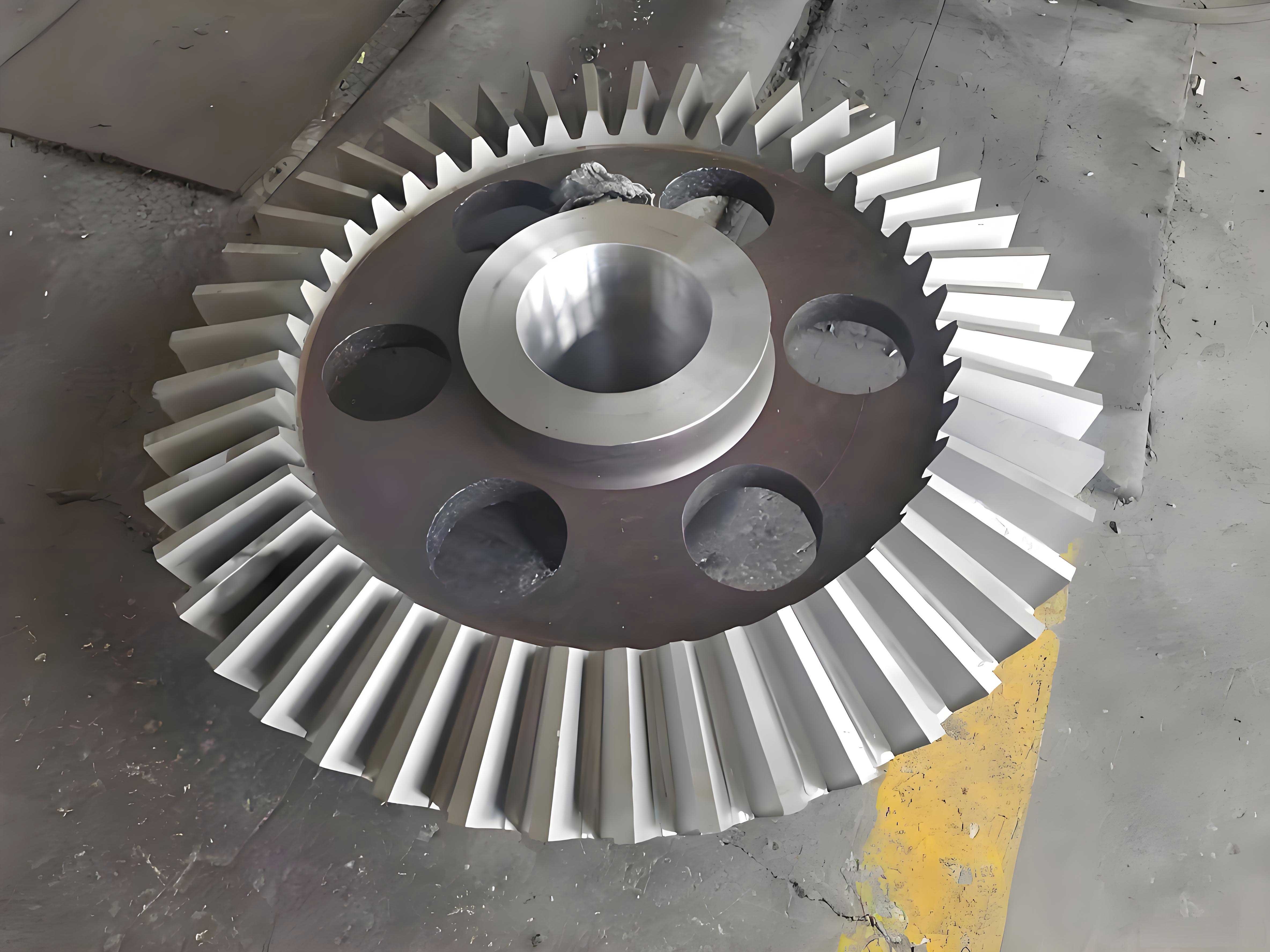
I began this work from a practical manufacturing problem: a double helical gear, also called a herringbone gear, must transmit heavy torque without generating net axial force, yet the conventional hobbing and grinding route forces a recess between the left-hand and right-hand helical sections. That recess increases axial length, reduces gearbox compactness, and weakens the alignment between the two helical halves. I therefore investigated a recess-free strategy based on multi-axis numerical control machining with general-purpose end mills. The same logic is relevant to miter gears and other angular gear forms, because miter gears also require careful flank control, tool orientation, and tool path planning when they are produced on multi-axis machines. In many small-batch applications, miter gears and double helical gears share the need for flexible machining rather than dedicated cutters.
My objective was not only to produce a recess-free double helical gear but also to optimize the finishing tool path so that the required accuracy could be reached with less machining time. I used side milling with a flat end mill for the involute helical flanks, ball end milling for the root fillets, and a constant scallop height strategy for the finishing passes. The constant scallop height method is especially attractive for miter gears and double helical gears because their flanks are curved surfaces whose local curvature changes along the profile. If the stepover is chosen from the smallest curvature radius, the rest of the surface is overmachined and the cycle time becomes unnecessarily long. I therefore developed a method to distribute finishing passes so that the residual height remains within tolerance while the stepover is maximized.
In this study I treated the gear as a pair of opposite-handed helical gears joined without a central groove. The left-hand and right-hand flanks cancel axial thrust during meshing, which is the main advantage of a double helical gear. The absence of a recess improves the continuity of the tooth root and gives better centering between the two helical sections. For miter gears, the axial thrust problem is different, but the need for accurate flank generation and efficient tool paths remains. I mention miter gears repeatedly because the optimization principles I developed can be adapted to miter gears when their flanks are machined by flank milling or five-axis contouring.
1. Geometric Model and Design Parameters
I first established a parametric model of the recess-free double helical gear. The gear had a normal module of 16 mm, 30 teeth, a pressure angle of 20 degrees, a helix angle of plus or minus 30 degrees, a addendum coefficient of 1.0, and a clearance coefficient of 0.25. The left-hand and right-hand halves were mirror images about the mid-plane. The main parameters are summarized in Table 1.
| Parameter | Symbol | Value | Unit |
|---|---|---|---|
| Normal module | $$m$$ | 16 | mm |
| Number of teeth | $$z$$ | 30 | — |
| Addendum coefficient | $$h_a^*$$ | 1.0 | — |
| Pressure angle | $$\alpha$$ | 20 | degree |
| Helix angle | $$\beta$$ | +30 / -30 | degree |
| Clearance coefficient | $$c^*$$ | 0.25 | — |
| Tooth width per half | $$b$$ | as designed | mm |
| Total gear width | $$B$$ | without recess | mm |
The transverse involute profile can be written in parametric form as
$$x = r_b(\cos\phi + \phi\sin\phi)$$
$$y = r_b(\sin\phi – \phi\cos\phi)$$
where $$r_b$$ is the base radius and $$\phi$$ is the involute roll angle. The quantity $$\phi$$ is related to the pressure angle $$\alpha$$ and the polar angle $$\theta$$ by
$$\phi = \theta + \alpha$$
For a helical gear, the transverse involute is swept along a helix. If the axial coordinate is $$z$$ and the lead is $$h$$, the helical surface can be expressed as
$$x = r_b[\cos(\phi+\mu) + \phi\sin(\phi+\mu)]$$
$$y = r_b[\sin(\phi+\mu) – \phi\cos(\phi+\mu)]$$
$$z = \frac{h}{2\pi}\mu$$
Here $$\mu$$ is the parameter along the helix. For a right-hand helix, $$\mu$$ increases in the positive $$z$$ direction. For a left-hand helix, the sign of $$\mu$$ is reversed. The helix angle on a cylinder of diameter $$d$$ satisfies
$$\tan\beta = \frac{\pi d}{h}$$
This relation is important for both double helical gears and miter gears. In miter gears, the pitch cone and tooth orientation create a different geometric family, but the same idea of a lead and a local helix angle appears in many spiral bevel and miter gear designs. I used this relation to generate the finishing tool paths from the discrete contact points.
2. Machining Strategy and Tool Selection
I selected a flank milling strategy for the involute helical surfaces and a ball end milling strategy for the root fillets. A flat end mill has a cylindrical cutting edge that can be aligned with the ruled nature of the involute helical flank. Because the flank is a convex surface and its curvature changes gradually, a flat end mill can remove material with a larger stepover than a ball end mill. This is a major advantage for miter gears as well, since miter gear flanks often have large curved regions where a ball end mill would require many closely spaced passes.
The tool material was PVD-coated solid carbide. The gear was made of carburized steel with a surface hardness in the range of HRC 58 to 62 and a core hardness in the range of HRC 30 to 40. Coated carbide provided better wear resistance and higher cutting speed than high-speed steel. I chose a 20 mm end mill for the upper part of the tooth slot, a 10 mm end mill for the narrower lower region, a 12 mm end mill for flank semi-finishing and finishing, and an 8 mm ball end mill for the root fillet. The tool data are given in Table 2.
| Operation | Tool type | Diameter | Material | Helix angle | Rake angle | Clearance angle |
|---|---|---|---|---|---|---|
| Roughing upper slot | Flat end mill | 20 mm | PVD carbide | 40 deg | 10 deg | 12 deg |
| Roughing lower slot | Flat end mill | 10 mm | PVD carbide | 30 deg | 10 deg | 12 deg |
| Flank semi-finishing | Flat end mill | 12 mm | PVD carbide | 30 deg | 10 deg | 15 deg |
| Flank finishing | Flat end mill | 12 mm | PVD carbide | 30 deg | 10 deg | 15 deg |
| Root semi-finishing and finishing | Ball end mill | 8 mm | PVD carbide | 30 deg | 10 deg | 15 deg |
The cutting parameters were chosen according to the tool material, the workpiece hardness, and the need to avoid chatter. The cutting speed was calculated from
$$v_c = \frac{\pi d n}{1000}$$
where $$v_c$$ is the cutting speed in m/min, $$d$$ is the tool diameter in mm, and $$n$$ is the spindle speed in r/min. The feed speed was calculated from
$$v_f = f n = z f_z n$$
where $$v_f$$ is the feed speed in mm/min, $$f$$ is the feed per revolution in mm/r, $$f_z$$ is the feed per tooth in mm/z, and $$z$$ is the number of teeth on the cutter. For roughing I used a feed per tooth of about 0.15 mm, and for finishing I used about 0.10 mm. The selected spindle speeds and feed speeds are listed in Table 3.
| Operation | Spindle speed (r/min) | Feed speed (mm/min) | Axial depth of cut (mm) | Radial width (mm) |
|---|---|---|---|---|
| Roughing with 20 mm end mill | 800–1200 | 500 | 5–7 | 3–5 |
| Roughing with 10 mm end mill | 800–1200 | 500 | 3–5 | 2–4 |
| Semi-finishing flanks with 12 mm end mill | 2300–3000 | 500 | 0.5–1.0 | 0.5–1.0 |
| Semi-finishing root with 8 mm ball mill | 2500 | 500 | 0.3–0.8 | 0.3–0.8 |
| Finishing flanks with 12 mm end mill | 2500 | 500 | 0.1–0.3 | 0.1–0.3 |
| Finishing root with 8 mm ball mill | 2500 | 500 | 0.1–0.2 | 0.1–0.2 |
The overall process sequence was roughing, semi-finishing, and finishing. In the roughing stage I used the 20 mm end mill for the wider upper portion of the slot and the 10 mm end mill for the lower portion. In the semi-finishing stage I used the 12 mm end mill for the flanks and the 8 mm ball end mill for the root. In the finishing stage I used the 12 mm end mill for the flanks and the 8 mm ball end mill for the root fillet. The process plan is shown in Table 4.
| Stage | Operation | Machining method | Tool | Purpose |
|---|---|---|---|---|
| 1 | Roughing open slot | Variable contour milling | 20 mm flat end mill | Remove bulk material above the lower slot region |
| 2 | Roughing slot bottom | Variable contour milling | 10 mm flat end mill | Remove material in the narrow bottom region |
| 3 | Flank semi-finishing | Variable contour milling | 12 mm flat end mill | Prepare the involute flanks with uniform stock |
| 4 | Root semi-finishing | Variable contour milling | 8 mm ball end mill | Prepare the root fillet region |
| 5 | Flank finishing | Variable contour milling | 12 mm flat end mill | Achieve final involute accuracy with constant scallop height |
| 6 | Root finishing | Variable contour milling | 8 mm ball end mill | Finish the root fillet and avoid cutter interference |
3. CAM Programming for the Recess-Free Geometry
I used a commercial CAD/CAM platform with an integrated CAM module. The gear model was created from the parameter table, and the CAM setup was built with a workpiece coordinate system whose origin coincided with the gear center. The safety plane was placed 100 mm above the tooth surface. The blank was a cylinder whose diameter was equal to the tip diameter and whose height was equal to the total gear width.
For the roughing operation I created an auxiliary plane near the middle of the slot and used a surface-driven variable contour milling operation. The drive surface was the auxiliary plane, the cutting direction was along the tooth trace, and the milling mode was zigzag. The projection vector was the tool axis, and the tool axis was set to four-axis relative to the drive body. This generated a tool path that removed the upper portion of the slot without causing interference. I then copied the operation and reduced the drive surface percentage to machine only the lower portion with the 10 mm end mill. This is important because the 20 mm end mill cannot reach the narrow bottom region without gouging.
For the flank semi-finishing operation I used the same variable contour milling strategy but selected the involute flank as the drive surface. The cutting direction was along the tooth trace, and the mode was zigzag. I set a positive offset in the surface drive method to leave finishing stock. For the root semi-finishing operation I selected the slot bottom surface and used the 8 mm ball end mill with an offset of about 1 mm. This prepared the root fillet for finishing.
For the flank finishing operation I used the 12 mm end mill with a single-direction cutting mode to maintain climb milling. The offset was set to zero so that the tool path followed the final flank surface. For the root finishing operation I used the 8 mm ball end mill and controlled the drive surface percentage so that only the root fillet was machined. I avoided using the center of the ball end mill as the contact point because the cutting speed approaches zero at the center, which causes poor surface finish and rapid tool wear. The same caution applies to miter gears when a ball end mill is used near the toe or heel of the tooth.
I verified each operation with a three-dimensional dynamic simulation inside the CAM environment. The simulation showed that the tool paths did not overcut the flanks and that the tool holder did not collide with the workpiece. The roughing and semi-finishing operations were straightforward, but the finishing operation required further optimization because the involute curvature changes from the root to the tip. I therefore applied the constant scallop height method to the flank finishing path.
4. Constant Scallop Height Method for the Finishing Path
The constant scallop height method aims to keep the residual height after machining as close as possible to a specified value. If the residual height is too small, the stepover is smaller than necessary and the machining time increases. If the residual height is too large, the gear may fail the accuracy requirement. For a double helical gear with a grade 6 accuracy requirement, I selected a scallop height of 0.0025 mm. The local curvature radius of the involute varies from the root to the tip. At the start of the involute the curvature radius is about 77.366 mm, and at the tip circle it is about 143.821 mm. This variation means that a constant parameter stepover must be chosen from the smallest curvature radius, which causes redundant passes near the tip.
For a convex surface approximated locally by a circle of radius $$r$$, the stepover $$l$$ for a specified scallop height $$\lambda$$ is given by
$$l = 2\sqrt{2r\lambda – \lambda^2}$$
For small $$\lambda$$, this can be approximated as
$$l \approx 2\sqrt{2r\lambda}$$
The relation shows that the stepover increases with the square root of the curvature radius. Therefore, if the curvature radius near the tip is almost twice the curvature radius near the root, the allowable stepover near the tip is about 1.4 times the stepover near the root. This is the source of the redundancy in constant parameter machining. The same relation is useful for miter gears, because miter gear flanks also exhibit varying local curvature along the tooth profile.
I calculated the stepover values for the involute flank at several curvature radii. The results are listed in Table 5. The stepover increases from about 1.24 mm near the root to about 1.70 mm near the tip. If a constant parameter method is used, the stepover must be limited to the smallest value, about 1.24 mm, over the entire flank. The constant scallop height method allows the stepover to increase gradually, which reduces the number of passes.
| Curvature radius (mm) | Scallop height (mm) | Stepover (mm) | Location on involute |
|---|---|---|---|
| 77.366 | 0.0025 | 1.244 | Near involute start |
| 90.000 | 0.0025 | 1.341 | Lower middle |
| 105.000 | 0.0025 | 1.449 | Middle |
| 120.000 | 0.0025 | 1.549 | Upper middle |
| 135.000 | 0.0025 | 1.643 | Near tip |
| 143.821 | 0.0025 | 1.696 | Tip circle |
I implemented the constant scallop height method by first selecting the tip circle as the initial contact curve. I offset the flank surface by the scallop height and intersected the offset surface with a tangent plane. The intersection curve gave the next constant scallop height curve. I repeated this process until the contact curves covered the entire flank. For the helical gear, the contact points were first computed in the transverse plane and then projected along the helix to form the three-dimensional tool path. The helix angle at each contact point was computed from the local diameter and the lead.
For a right-hand helical flank, the tool path was generated by rotating each transverse contact point through the helix parameter $$\mu$$. The axial position was
$$z = \frac{h}{2\pi}\mu$$
The radial position was determined by the involute equations. For a left-hand flank, the sign of $$\mu$$ was reversed. I used the same procedure for both halves of the recess-free double helical gear. The transition at the mid-plane was continuous because no recess was present.
The constant scallop height method produced 21 finishing passes per flank. The constant parameter method required 25 passes per flank. The difference is four passes per flank. For a gear with 30 teeth and two flanks per tooth, this represents a significant reduction in finishing time. The comparison is shown in Table 6.
| Method | Finishing passes per flank | Total finishing passes for one gear | Relative pass count |
|---|---|---|---|
| Constant parameter | 25 | 25 × 2 × 30 = 1500 | 100% |
| Constant scallop height | 21 | 21 × 2 × 30 = 1260 | 84% |
The stepover values from the constant scallop height calculation are listed in Table 7. The first stepover near the tip was about 1.686 mm, and the last stepover near the root was about 1.235 mm. The stepover decreased gradually as the curvature radius decreased. This is the opposite of the constant parameter method, where the stepover is fixed at the minimum value. The constant scallop height method therefore avoids redundant passes near the tip while maintaining the required residual height near the root.
| Stepover number | Stepover value (mm) | Region |
|---|---|---|
| 1 | 1.6864 | Tip side |
| 3 | 1.6499 | Upper flank |
| 6 | 1.5908 | Upper middle |
| 10 | 1.5063 | Middle |
| 14 | 1.4094 | Lower middle |
| 18 | 1.2989 | Lower flank |
| 20 | 1.2346 | Root side |
The constant scallop height method is not limited to double helical gears. I believe it can also improve the finishing of miter gears, especially when the miter gears are machined on five-axis machine tools and the flanks are generated by side milling. In miter gears, the local curvature and the tool orientation change from the toe to the heel, and a constant scallop height strategy can reduce the number of redundant passes. The same mathematical framework can be adapted to miter gears by replacing the involute helicoid with the appropriate miter gear flank surface.
5. Secondary Development for Automatic Tool Path Generation
The constant scallop height calculation is mathematically straightforward but tedious if it is performed manually for every flank. I therefore developed a secondary development program to automate the generation of the finishing tool path. The program was built inside the CAD/CAM platform using its knowledge fusion language and its menu and dialog tools. The goal was to let the user select the contact points, set the helix parameters, and generate the finishing path automatically.
I first created a user menu in the CAD/CAM environment. The menu contained a single command that opened the constant scallop height finishing dialog. I added a message that explained the function of the command. I then designed a user interface with three groups. The first group allowed the user to select the contact points that had been imported from the external calculation. The second group allowed the user to set the base radius, the helix angle, the contact point radius, and the lead. The third group displayed a schematic of the finishing path so that the user could understand the result before generating the path.
I considered two secondary development strategies. The first was a modeling method. In this method the software creates a tangent plane at the initial contact curve, offsets the flank surface by the scallop height, intersects the offset surface with the tangent plane, and uses the intersection curve as the next contact curve. This process is repeated until the flank is covered. The modeling method is intuitive for a straight cylindrical gear, but it is not directly suitable for a helical gear because the contact curve must be a helix. The second strategy was a point-line method. In this method the contact points are computed in the transverse plane, and each contact point is then used to generate a helix. The point-line method is more general and can be used for both straight gears and helical gears. I therefore chose the point-line method.
| Development method | Principle | Suitable gear type | Advantage | Limitation |
|---|---|---|---|---|
| Modeling method | Offset surface, tangent plane, intersection curve | Straight cylindrical gears | Directly uses solid geometry | Not directly suitable for helical flanks |
| Point-line method | Compute contact points, generate helices | Straight and helical gears | General and programmable | Requires external point calculation |
I used an external mathematical program to compute the contact points. The input was the involute equation, the base radius, the tip radius, the start radius, and the specified scallop height. The output was a set of contact points in the transverse plane. I imported these points into the CAD/CAM environment and used the knowledge fusion program to generate a helix through each point. The helix angle was computed from
$$\beta = \arctan\left(\frac{\pi d}{h}\right)$$
where $$d$$ is the local diameter and $$h$$ is the lead. The program then offset each contact point by the tool radius along the normal direction of the involute. The final tool path was obtained by connecting the offset points along the helix. This produced a smooth finishing path that respected the constant scallop height condition.
The secondary development program reduced the programming time from several hours to a few minutes. It also reduced the chance of manual error. The user could change the scallop height and immediately see how the number of passes changed. This is useful for miter gears as well, because miter gear designers often need to evaluate several tool path strategies before committing to a production process. A similar point-line method can be used for miter gears if the miter gear flank is represented by a suitable parametric surface.
6. Verification by Machining Simulation
Before machining the actual gear, I verified the numerical control programs with a machining simulation environment. I built models of the cutting tools, the tool holders, the fixture, and the workpiece. I imported the machine tool kinematic model and set the travel limits, the initial position, and the collision detection rules. I then loaded the numerical control programs and ran the simulation.
The simulation confirmed that the tool paths did not overcut the flanks and that the tool holder did not collide with the workpiece or the fixture. The simulation also allowed me to compare the constant parameter finishing path with the constant scallop height finishing path. The simulated machining time for one flank with the constant parameter method was 24 minutes and 22 seconds. The simulated machining time for one flank with the constant scallop height method was 19 minutes and 4 seconds. The constant scallop height method saved about 5 minutes and 18 seconds per flank in simulation. The results are listed in Table 8.
| Method | Simulated time per flank | Simulated time per tooth | Simulated time for 30 teeth |
|---|---|---|---|
| Constant parameter | 24 min 22 s | 48 min 44 s | 24 h 22 min |
| Constant scallop height | 19 min 4 s | 38 min 8 s | 19 h 4 min |
| Difference | 5 min 18 s | 10 min 36 s | 5 h 18 min |
The simulation gave me confidence that the constant scallop height path was not only shorter but also safe. I also used the simulation to check the root finishing operation. The ball end mill approach was adjusted to avoid contact near the center of the tool. The simulation showed that the root fillet was machined without interference. For miter gears, a similar simulation step is essential because the tool orientation changes rapidly near the heel and toe, and collision checking is more critical than for a parallel-axis gear.
7. Machining Experiment and Measurement
I machined the recess-free double helical gear on a five-axis turn-mill machining center. The machine had a large rotary table and a powerful spindle, which allowed the gear to be machined in one setup. I designed a fixture that supported the gear blank and prevented rotation during cutting. A keyway and a parallel key were used to restrict the rotational degree of freedom. I measured the runout of the blank and adjusted it to within 0.01 mm. I then ran the roughing, semi-finishing, and finishing programs. For the finishing stage I used two different programs on different flanks: one based on the constant parameter method and one based on the constant scallop height method. I recorded the actual machining time for each method.
The actual machining time for one flank with the constant parameter method was 31 minutes and 30 seconds. The actual machining time for one flank with the constant scallop height method was 25 minutes and 36 seconds. For one tooth, which has two flanks, the constant parameter method required 63 minutes, and the constant scallop height method required 51 minutes and 12 seconds. For 30 teeth, the constant scallop height method saved 5 hours and 54 minutes, which is about 19 percent of the finishing time. The comparison is shown in Table 9.
| Method | Actual time per flank | Actual time per tooth | Actual time for 30 teeth | Relative time |
|---|---|---|---|---|
| Constant parameter | 31 min 30 s | 63 min | 31 h 30 min | 100% |
| Constant scallop height | 25 min 36 s | 51 min 12 s | 25 h 36 min | 81% |
| Difference | 5 min 54 s | 11 min 48 s | 5 h 54 min | 19% |
The actual machining time was longer than the simulated time because the operator checked the tool, adjusted the coolant, and changed the tool when necessary. The trend, however, matched the simulation. The constant scallop height method was consistently faster. This confirmed that the optimized tool path was effective in practice.
I also compared the numerical control method with the traditional method. The traditional method uses a hob for roughing and a grinding wheel for finishing. It requires a recess between the left-hand and right-hand helices. The traditional method is faster in pure cutting time, about 50 hours for this gear, while the numerical control method required about 80 hours. However, the traditional method requires a custom hob and a custom grinding wheel. The lead time for those tools is often several weeks. The numerical control method uses standard end mills, which can be purchased immediately. For small-batch production of miter gears, double helical gears, and other custom gear types, the numerical control method is therefore more flexible. The comparison is shown in Table 10.
| Method | Cutting time | Tooling lead time | Flexibility | Suitable production scale |
|---|---|---|---|---|
| Traditional hobbing and grinding | About 50 h | Several weeks for custom tools | Low for different modules and pressure angles | Large batch |
| Numerical control flank milling | About 80 h | Standard tools available immediately | High for different modules and pressure angles | Small and medium batch |
After machining I measured the gear on a gear measuring instrument. The instrument compared the measured flank with a master model built from the gear parameters. The measurement items included total profile deviation, profile form deviation, profile slope deviation, total helix deviation, helix form deviation, and helix slope deviation. The results are listed in Table 11.
| Measurement item | Maximum value (μm) | Minimum value (μm) | Average value (μm) | Grade 6 limit (μm) |
|---|---|---|---|---|
| Total profile deviation | 11.3 | 7.6 | 9.7 | 23 |
| Profile form deviation | 9.2 | 3.8 | 5.8 | 18 |
| Profile slope deviation | 10.0 | 5.7 | 7.6 | ±15 |
| Total helix deviation | 11.5 | 10.3 | 10.8 | 18 |
| Helix form deviation | 3.3 | 2.6 | 3.0 | 13 |
| Helix slope deviation | 11.7 | 10.5 | 11.1 | ±13 |
All measured values were within the grade 6 limits. The total profile deviation reached a maximum of 11.3 μm, and the total helix deviation reached a maximum of 11.5 μm. The helix slope deviation reached 11.7 μm, which is close to the limit of ±13 μm but still acceptable. The measurement confirmed that the constant scallop height finishing path produced a flank that met the design requirement.
I analyzed the helix slope deviation because it was the largest item. Three factors may have contributed. First, the helix used to generate the tool path may not have been modeled with sufficient precision. Second, the gear model itself may have had a small helix error. Third, the fixture used a key connection, and the clearance in the keyway may have allowed a small rotational error. These factors can be reduced by improving the helix model, replacing the tool more frequently, and using a more rigid fixture. The same analysis applies to miter gears, where the helix or spiral angle is often the most sensitive measurement item.
8. Discussion and Practical Implications
The results show that a recess-free double helical gear can be machined on a multi-axis numerical control machine with standard end mills. The absence of a recess improves the compactness of the gearbox and the alignment between the left-hand and right-hand helices. It also improves the bending strength of the root because the material is continuous across the mid-plane. The method is flexible because the same tool set can be used for different modules, teeth numbers, and pressure angles. This flexibility is valuable for miter gears and other custom gear types, where dedicated tooling is expensive and slow to obtain.
The constant scallop height method is the key to reducing the finishing time. The involute flank has a curvature radius that changes from the root to the tip. A constant parameter method must use the smallest stepover over the entire flank, which creates redundant passes near the tip. The constant scallop height method adjusts the stepover locally so that the residual height remains within tolerance while the stepover is as large as possible. This reduced the number of finishing passes from 25 to 21 per flank and saved about 19 percent of the finishing time in the actual machining experiment. For miter gears, the same principle can reduce redundant passes on the tooth flank and improve the efficiency of five-axis finishing.
The secondary development program made the constant scallop height method practical. Without automation, the calculation of contact points and the generation of helices would be too slow for production use. The program allowed the user to select contact points, set the helix parameters, and generate the finishing path automatically. The point-line method was chosen because it works for both straight and helical gears. The same program structure can be adapted to miter gears by changing the contact point calculation and the flank surface representation.
The simulation and experiment confirmed the accuracy of the numerical control programs. The simulation predicted the tool path length and the machining time with reasonable accuracy. The actual machining time was longer because of operator checks and tool changes, but the relative improvement of the constant scallop height method was preserved. The measurement showed that the gear met grade 6 accuracy. The largest deviations were in the helix direction, which suggests that the helix model and the fixture rigidity should be improved in future work.
9. Conclusions
I developed a complete process for machining a recess-free double helical gear on a multi-axis numerical control machine. The process uses standard end mills for roughing and flank finishing and a ball end mill for the root fillet. The absence of a recess improves compactness, alignment, and root strength. The method is flexible for small-batch production of different gear sizes and is suitable for miter gears and other custom gear forms.
I optimized the flank finishing path with the constant scallop height method. The method produced 21 passes per flank instead of 25 passes for the constant parameter method. In actual machining, the optimized path reduced the finishing time by about 19 percent, saving about 5 hours and 54 minutes for the 30-tooth gear. The measurement confirmed that the gear met grade 6 accuracy requirements.
I also developed a secondary development program that automates the constant scallop height tool path generation. The program uses a point-line method, which is suitable for both straight and helical gears. The program reduces programming time and manual error. The same approach can be extended to miter gears, where the tool path optimization has similar economic value.
10. Future Work
Several improvements remain for future work. First, the ball end mill path for the root fillet should be further optimized. The tool axis should be adjusted so that the contact point stays away from the center of the ball end mill. This will improve the surface finish and reduce tool wear. Second, the finishing strategy could combine climb milling and conventional milling. Climb milling gives better surface quality, but conventional milling may reduce the path length in some regions. The accuracy of the conventional milling regions must be tested. Third, the method should be extended to gears with profile modification and helix modification. In that case, the flank surface is no longer a standard involute helicoid, and the contact point calculation must include the modification. Fourth, the same constant scallop height logic should be applied to miter gears and other angular gear types. Miter gears often require five-axis machining, and the tool path optimization can reduce cost and lead time.
Overall, I found that recess-free double helical gear machining with constant scallop height tool path optimization is a practical and effective alternative to traditional hobbing and grinding for small-batch production. The method can also provide useful guidance for miter gears and other complex gear geometries that must be machined on multi-axis machine tools.