
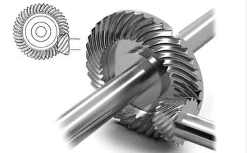
I centered my research on the reconstruction and computer numerical control machining of spiral bevel gears because these components remain among the most critical and most difficult parts in automotive, heavy machinery, aerospace, and industrial transmission systems. A spiral bevel gear pair transmits motion between intersecting axes with high load capacity, smooth engagement, and relatively low noise. However, its tooth surface geometry is complex, and its manufacturing quality directly affects vibration, fatigue life, contact stress, and transmission accuracy. In my work, I did not begin with a conventional cutting machine or a dedicated gear grinder. Instead, I started from the digital model of the spiral bevel gear and asked whether the geometric smoothness of the tooth surface could be improved before machining. My central idea was to combine spherical involute theory, non-uniform rational B-spline surfaces, wavelet multiresolution analysis, and universal CNC machining. Through this combination, I aimed to reduce surface complexity, suppress overcut, and improve the final machining accuracy of the spiral bevel gear tooth surface.
1. Research Motivation and Problem Statement
My motivation came from the growing demand for spiral bevel gears in vehicle drivetrains, excavators, cranes, bulldozers, and other heavy-duty machines. The performance requirements for these machines include higher reliability, longer durability, lower noise, and better transmission stability. At the same time, product development has shifted toward shorter cycles, smaller batches, and greater variety. Conventional spiral bevel gear manufacturing depends heavily on dedicated machines and dedicated cutters. Although such methods can produce acceptable gears, they also create several problems that I wanted to address.
The first problem is the principle-level limitation of conjugate surface design. Many traditional spiral bevel gear models are based on conjugate surface theory, and the resulting tooth profile is only an approximation of a spherical involute. This approximation introduces a principle error, which can lead to unstable instantaneous transmission ratio, uneven contact stress, and noise. The second problem is manufacturing flexibility. A dedicated machine is efficient for one family of parts, but it is not flexible for rapid product changes. The third problem is the cost of accuracy. To reach high accuracy, companies often rely on repeated trial cuts, machine parameter corrections, and post-processing such as grinding, lapping, or electrochemical finishing. These steps increase equipment investment and production time.
I therefore formulated my research around a different question: can I improve the machining accuracy of a spiral bevel gear by optimizing its digital tooth surface before machining? In particular, I asked whether wavelet-based multiresolution processing could remove high-frequency geometric details that are difficult for a CNC machine to follow, while preserving the overall shape and fitting accuracy of the spiral bevel gear tooth surface. If this is possible, then the digital model itself can become a tool for improving machining quality, not merely a passive reference.
| Problem in Conventional Spiral Bevel Gear Manufacturing | My Proposed Direction |
|---|---|
| Principle error from approximate conjugate surfaces | Use spherical involute theory as the tooth profile basis |
| Dedicated machines and cutters reduce flexibility | Use universal multi-axis CNC machining |
| High accuracy often requires costly post-processing | Optimize the digital tooth surface before machining |
| Complex surface details cause overcut and vibration | Apply wavelet multiresolution decomposition and reconstruction |
| Fitting accuracy and surface smoothness are often in conflict | Balance them by removing high-frequency control-point information |
2. Mathematical Foundation of the Spiral Bevel Gear Tooth Surface
2.1 Spherical Involute Theory
I used spherical involute theory as the geometric foundation of the spiral bevel gear tooth surface. In a spherical involute, every point on the tooth profile remains on a sphere whose center is the apex of the base cone. During meshing, the instantaneous transmission ratio remains constant, and the contact is theoretically a line contact. This is advantageous for reducing noise and improving stress distribution. The spherical involute is generated when a rolling plane rolls without slipping on a base cone. A fixed point on the rolling plane traces the involute on the sphere.
Let the base cone angle be \(\delta_b\), and let the rolling parameter be \(\beta\). In the moving coordinate system \(O’X’Y’Z’\), the position of a point on the generating line can be written as
$$
\begin{cases}
x’ = l \sin \psi \\
y’ = 0 \\
z’ = l \cos \psi \\
\psi = \beta \sin \delta_b
\end{cases}
$$
Here, \(l\) is the distance from the cone apex to the point, and \(\psi\) is the angular parameter on the cone surface. The coordinate transformation from the moving system to the fixed system can be expressed as
$$
\begin{bmatrix}
x \\ y \\ z
\end{bmatrix}
=
\begin{bmatrix}
\sin\beta & \cos\beta & 0 \\
-\cos\delta_b \cos\beta & -\cos\delta_b \sin\beta & -\sin\delta_b \\
\sin\delta_b \cos\beta & \sin\delta_b \sin\beta & \cos\delta_b
\end{bmatrix}
\begin{bmatrix}
x’ \\ y’ \\ z’
\end{bmatrix}
$$
By changing \(\beta\) and \(l\), I obtained different points on the spherical involute. When the starting points on the base cone form a straight line along the generatrix, the result is a straight bevel gear. When they form an inclined line, the result is a skew bevel gear. When they form a spiral line, the result is a spiral bevel gear. This is the key reason I introduced a spiral line into the model.
2.2 Spiral Line Based on the Cutting Principle
To retain the characteristic geometry of a cut spiral bevel gear, I designed the spiral line according to the cutting principle. I considered a cutter disk rotating with angular velocity \(\omega_1\) while the workpiece rotates with angular velocity \(\omega_2\). The combined motion of a point on the cutter disk produces a straight line in the fixed reference frame. The trajectory of point \(A\) on the cutter disk can be written as
$$
\begin{cases}
x = 2r \sin(\omega t) \\
y = 0 \\
z = 0
\end{cases}
$$
where \(r\) is the cutter radius. For the rolling contact between the base cone and the rolling plane, the linear velocities at the common tangent point must be equal. Therefore,
$$
\omega_2 = \frac{\omega}{\sin \delta_b}
$$
This relation ensures that the straight-line trajectory of the cutter point is imprinted on the base cone as a spiral line. In my model, the cutter radius was selected according to the outer cone distance \(L_a\). For a face width coefficient of \(1/3\), I used
$$
r = \frac{5}{6} L_a
$$
In this way, the spiral bevel gear model retained a cutting-like spiral direction while still being defined analytically and parametrically.
2.3 Example Spiral Bevel Gear Pair
I selected a zero-modified spiral bevel gear pair as my computational example. The main parameters are listed in Table 1. These values were used to generate discrete points on both the concave and convex tooth surfaces.
| Parameter | Wheel | Pinion |
|---|---|---|
| Number of teeth \(Z\) | 43 | 11 |
| Large-end module \(m_s\) | 4.65 mm | 4.65 mm |
| Pressure angle \(\alpha\) | 20 degrees | 20 degrees |
| Mean spiral angle \(\beta_m\) | 30 degrees | 30 degrees |
| Shaft angle \(\Sigma\) | 90 degrees | 90 degrees |
| Addendum coefficient \(f\) | 0.85 | 0.85 |
| Clearance coefficient \(c\) | 0.188 | 0.188 |
| Pitch diameter \(d\) | 199.95 mm | 51.15 mm |
| Pitch cone angle \(\delta\) | 75.6507 degrees | 14.3493 degrees |
| Outer cone distance \(L_a\) | 103.1945 mm | 103.1945 mm |
| Circular pitch \(t\) | 14.6084 mm | 14.6084 mm |
| Addendum \(h’\) | 3.4875 mm | 3.4875 mm |
| Dedendum \(h”\) | 4.8267 mm | 4.8267 mm |
| Whole depth \(h\) | 8.3142 mm | 8.3142 mm |
| Root angle \(\delta_b\) | 72.975 degrees | 11.674 degrees |
| Face angle \(\delta_a\) | 78.326 degrees | 17.025 degrees |
| Theoretical arc tooth thickness \(S\) | 7.3042 mm | 7.3042 mm |
I wrote a complete calculation program to generate the discrete points. The concave and convex surfaces are similar in structure, but they differ in the starting angle on the root cone and in the rolling direction. In my program, I reversed the sign of the angular parameter in the transformation matrix to obtain the opposite surface. For each tooth surface, I generated 55 discrete points initially, but the number of points can be adjusted according to the required fitting accuracy.
2.4 Discrete Point Generation
My point generation procedure can be summarized as follows:
- Define the basic spiral bevel gear parameters: teeth number, module, pressure angle, spiral angle, cone angles, and face width.
- Compute the base cone angle, root angle, face angle, and outer cone distance.
- Select a set of radial positions \(l\) along the tooth width.
- Select a set of angular positions \(\beta\) along the involute direction.
- Apply the spherical involute equations.
- Apply the coordinate transformation to the fixed gear coordinate system.
- Apply the spiral line relation to obtain the spiral bevel gear tooth surface.
- Separate the concave and convex surfaces by changing the rolling direction and starting angle.
This procedure gave me a parametric and repeatable way to build a spiral bevel gear tooth surface without relying on an approximate conjugate surface. It also provided the input data for the next stage, which was NURBS fitting and wavelet optimization.
3. NURBS and Wavelet-Based Tooth Surface Reconstruction
3.1 Cubic NURBS Surface Fitting
I used cubic NURBS surfaces to fit the discrete points of the spiral bevel gear tooth surface. NURBS has excellent local controllability and can represent complex free-form surfaces with high precision. The general NURBS surface equation is
$$
S(u,v)=\frac{\sum_{i=0}^{n}\sum_{j=0}^{m} W_{i,j} V_{i,j} N_{i,3}(u) N_{j,3}(v)}{\sum_{i=0}^{n}\sum_{j=0}^{m} W_{i,j} N_{i,3}(u) N_{j,3}(v)}
$$
where \(W_{i,j}\) are the weights, \(V_{i,j}\) are the control points, and \(N_{i,3}(u)\) and \(N_{j,3}(v)\) are the cubic B-spline basis functions. The basis functions are defined recursively by the Cox-de Boor formula:
$$
N_{i,0}(u)=
\begin{cases}
1, & u_i \leq u < u_{i+1} \\
0, & \text{otherwise}
\end{cases}
$$
$$
N_{i,p}(u)=\frac{u-u_i}{u_{i+p}-u_i} N_{i,p-1}(u) + \frac{u_{i+p+1}-u}{u_{i+p+1}-u_{i+1}} N_{i+1,p-1}(u)
$$
For a cubic NURBS surface that passes through the first and last points, I used a knot vector with multiplicity four at both ends:
$$
U=\{0,0,0,0,u_4,u_5,\ldots,u_n,1,1,1,1\}
$$
$$
V=\{0,0,0,0,v_4,v_5,\ldots,v_m,1,1,1,1\}
$$
The fitting procedure I used had four main steps. First, I computed the knot vectors from the accumulated chord length. Second, I calculated the weight factors. Third, I constructed and solved the interpolation equations for the control points. Fourth, I repeated the procedure in the other parametric direction to obtain the control net of the spiral bevel gear tooth surface.
3.2 Wavelet Multiresolution Representation
After obtaining the NURBS tooth surface, I applied wavelet multiresolution analysis. The main idea is that any complex surface can be decomposed into a low-frequency base surface and one or more high-frequency detail surfaces. The low-frequency surface represents the main shape of the spiral bevel gear tooth, while the high-frequency surfaces represent small geometric details. These details often have high curvature and can cause vibration or overcut during CNC machining.
If the original surface is \(S_L(u,v)\), I can decompose it as
$$
S_L(u,v)=S_{L-1}(u,v)+G_{L-1}(u,v)
$$
where \(S_{L-1}(u,v)\) is the low-frequency smooth surface and \(G_{L-1}(u,v)\) is the high-frequency detail. In terms of B-spline basis functions, the decomposition can be written using matrices:
$$
\mathbf{N}^{i-1}_u = \mathbf{N}^{i}_u \mathbf{A}_i, \quad \mathbf{M}^{i-1}_u = \mathbf{N}^{i}_u \mathbf{B}_i
$$
Here, \(\mathbf{A}_i\) and \(\mathbf{B}_i\) are decomposition matrices. The corresponding reconstruction relation is
$$
\begin{bmatrix} \mathbf{P}_i & \mathbf{Q}_i \end{bmatrix}
\begin{bmatrix} \mathbf{A}_i \\ \mathbf{B}_i \end{bmatrix}
= \mathbf{E}
$$
For the control points, the decomposition can be expressed as
$$
\begin{bmatrix}
V^{L-1} \\
D^{L-1}
\end{bmatrix}
=
\begin{bmatrix}
P_1 & P_2 \\
Q_1 & Q_2
\end{bmatrix}
\begin{bmatrix}
V^{L} \\
D^{L}
\end{bmatrix}
$$
where \(V^{L-1}\) are the low-frequency control points and \(D^{L-1}\) are the detail control points. To remove high-frequency information, I set the detail control points to zero and reconstructed the control net. The resulting surface is smoother and has lower curvature, but it still retains the main shape of the spiral bevel gear tooth surface.
3.3 Optimization Procedure
My wavelet-based optimization procedure for the spiral bevel gear tooth surface was as follows:
- Fit the original discrete points with a cubic NURBS surface.
- Extract the control net and weights.
- Decompose the control net into low-frequency and high-frequency components.
- Set the high-frequency detail control points to zero.
- Reconstruct the control net.
- Generate the smoothed NURBS surface.
- Compare the smoothed surface with the original surface in terms of fitting error and Gaussian curvature.
This procedure does not simply smooth the surface blindly. It removes only the high-frequency details that are not essential to the overall spiral bevel gear geometry. In this way, the fitting accuracy remains acceptable while the surface becomes easier to machine.
3.4 Model Assembly and Interference Check
I imported the reconstructed NURBS surfaces into a CAD environment, arrayed them around the gear axis, added the hub and shaft hole, and assembled the wheel and pinion into a pair. I then performed a motion simulation to check for interference. The assembly showed no interference during the meshing cycle. I also simulated the contact region by introducing a very small interference allowance to represent elastic deformation. The contact region appeared as an elliptical patch, which is consistent with the expected contact behavior of a spiral bevel gear pair. This confirmed that the reconstructed tooth surfaces were suitable for further machining analysis.
3.5 Fitting Error and Gaussian Curvature Analysis
I compared the fitting error of the original tooth surface and the wavelet-optimized tooth surface. For each surface, I sampled 50 points and calculated the maximum and average fitting errors. The results are shown in Table 2.
| Surface | Maximum Error, Original | Average Error, Original | Maximum Error, Wavelet | Average Error, Wavelet |
|---|---|---|---|---|
| Wheel concave | 6.316 μm | 5.371 μm | 6.693 μm | 6.413 μm |
| Wheel convex | 18.672 μm | 6.693 μm | 20.594 μm | 7.532 μm |
| Pinion concave | 16.851 μm | 10.237 μm | 18.039 μm | 13.462 μm |
| Pinion convex | 6.254 μm | 5.623 μm | 13.065 μm | 15.256 μm |
The wavelet-optimized surfaces have larger fitting errors than the original surfaces. This is expected because removing high-frequency details changes the surface slightly. However, the fitting error remains on the order of several micrometers to about twenty micrometers, which is small compared with the machining error that will be discussed later. More importantly, the wavelet-optimized surfaces have lower Gaussian curvature and a smaller curvature range, as shown in Table 3.
| Tooth Surface | Original Gaussian Curvature Range | Wavelet Gaussian Curvature Range |
|---|---|---|
| Wheel concave | Maximum 0, minimum \(-2.56 \times 10^{-3}\), range \(2.56 \times 10^{-3}\) | Maximum \(-0.02 \times 10^{-3}\), minimum \(-1.74 \times 10^{-3}\), range \(1.72 \times 10^{-3}\) |
| Wheel convex | Maximum \(3.19 \times 10^{-3}\), minimum 0, range \(3.19 \times 10^{-3}\) | Maximum \(2.16 \times 10^{-3}\), minimum \(0.03 \times 10^{-3}\), range \(2.13 \times 10^{-3}\) |
| Pinion concave | Maximum \(-0.26 \times 10^{-3}\), minimum \(-3.98 \times 10^{-3}\), range \(3.72 \times 10^{-3}\) | Maximum \(-0.34 \times 10^{-3}\), minimum \(-3.14 \times 10^{-3}\), range \(2.80 \times 10^{-3}\) |
| Pinion convex | Maximum \(9.04 \times 10^{-3}\), minimum \(-0.88 \times 10^{-3}\), range \(9.92 \times 10^{-3}\) | Maximum \(6.04 \times 10^{-3}\), minimum \(-0.85 \times 10^{-3}\), range \(6.89 \times 10^{-3}\) |
The reduction in curvature range means that the surface is smoother and less complex. I regard this as the main advantage of the wavelet method. In CNC machining, a smoother spiral bevel gear tooth surface with lower curvature allows more stable tool motion and reduces the chance of sudden changes in cutting direction. It also permits a higher feed rate for the same allowable contour error. If the maximum contour error is \(\delta_{\max}\), the interpolation period is \(T_s\), and the curvature radius at a point is \(\rho_i\), then the feed rate \(v_i\) should satisfy
$$
v_i \leq \sqrt{2 a_{\max} \rho_i}
$$
$$
v_i \leq \frac{2}{T_s} \sqrt{2 \delta_{\max} \rho_i – \delta_{\max}^2}
$$
Since the wavelet-optimized surface has larger curvature radii, the allowable feed rate can be higher under the same error constraint. This is beneficial for both accuracy and efficiency.
4. Simulation of NC Machining on Universal CNC Machines
4.1 Machining Strategy and Workflow
I used a general-purpose CAD/CAM environment to simulate the machining of the spiral bevel gear. My workflow included blank design, turning of the blank, rough milling, semi-finish milling, finish milling, and post-processing. The main objective was to design a machining plan that could be executed on a universal CNC machine rather than a dedicated gear cutting machine.
For the finishing stage, I paid special attention to tool path continuity. I compared two basic path strategies: paths parallel to the tooth tip and paths parallel to the tooth root. The results are summarized in Table 4.
| Tool Path Strategy | Continuity | Risk of Overcut | Machining Efficiency | My Assessment |
|---|---|---|---|---|
| Parallel to tooth tip | Often interrupted near the root | Higher | Lower due to frequent retracts | Not preferred |
| Parallel to tooth root | Continuous | Lower | Higher | Preferred for finishing |
For the spiral bevel gear pinion, the tooth surface is more complex than the wheel. A three-axis machine cannot complete the entire pinion surface because of interference and blind areas. Therefore, I used a five-axis simulation strategy for the pinion. For the wheel, I compared three-axis and five-axis strategies to understand the limits of a universal three-axis CNC machine.
4.2 Pinion Machining Simulation
I treated the pinion as a blade-like part because its geometry is similar to an impeller without splitter blades. I used a multi-blade machining module. The steps were:
- Set the machining coordinate system and align it with the workpiece coordinate system.
- Define the multi-blade geometry: root cone, top cone, concave surface, convex surface, small end face, and fillet.
- Create the required cutters.
- Create roughing, semi-finishing, and finishing operations.
- Select the drive method and cutting layer mode.
- Determine the tool diameter from the minimum clearance between the concave and convex surfaces.
- Array the tool path around the pinion axis.
- Check the remaining allowance and overcut.
The minimum distance between the concave and convex surfaces near the root was about 2.2736 mm. Therefore, I selected a D4 ball-nose cutter for roughing and a D2 ball-nose cutter for semi-finishing. For finishing, I used a D2 cutter for the tooth surface and a D1 cutter for the hub surface where the space is narrow. The operations and tools are listed in Table 5.
| Operation | Tool | Purpose | Allowance or Target |
|---|---|---|---|
| Roughing | D4 ball-nose | Remove most material | 0.5 mm allowance |
| Semi-finishing | D2 ball-nose | Prepare for finishing | 0.2 mm allowance |
| Hub finishing | D1 ball-nose | Finish root cone surface | Residual height less than 0.02 mm |
| Fillet finishing | D2 ball-nose | Finish transition fillet | Residual height less than 0.02 mm |
| Tooth surface finishing | D2 ball-nose | Finish concave and convex surfaces | Residual height less than 0.02 mm |
The stepover was determined from the allowable scallop height. For a ball-nose cutter of radius \(R\) and stepover \(S\), the scallop height \(H\) is
$$
H = R – \sqrt{R^2 – \left(\frac{S}{2}\right)^2}
$$
For a maximum scallop height of 0.02 mm, a D2 cutter requires a stepover of about 0.398 mm, while a D1 cutter requires a stepover of about 0.279 mm. I used these values to set the finishing stepover. The cutting parameters for pinion simulation are listed in Table 6.
| Parameter | Roughing | Semi-Finishing | Finishing |
|---|---|---|---|
| Spindle speed | 2000 r/min | 2500 r/min | 3000 r/min |
| Feed rate | 250 mm/min | 200 mm/min | 150 mm/min |
| Stepover | 1.0 mm | 0.6 mm | 0.398 mm for D2, 0.279 mm for D1 |
| Allowance | 0.5 mm | 0.2 mm | 0 mm target |
| Drive method | Along blade, zigzag | Along blade, zigzag | Along blade, zigzag |
When I set the tangential and radial extensions to zero, the finishing path stopped before reaching the boundary, causing a large remaining allowance at the small end of the concave surface and the large end of the convex surface. I therefore added 1 mm of tangential and radial extension. After this correction, the pinion could be finished completely in simulation, with only a small residual region above the target scallop height.
4.3 Wheel Machining Simulation
The wheel is less complex than the pinion. I simulated both three-axis and five-axis finishing. The three-axis machine could complete the wheel surface, but the allowance distribution was less uniform. The five-axis machine produced a smaller and more uniform allowance. The comparison is given in Table 7.
| Machine Type | Maximum Allowance | Maximum Overcut | Allowance Uniformity | My Assessment |
|---|---|---|---|---|
| Three-axis | 0.338 mm | \(-0.2902\) mm | Less uniform | Possible but not optimal |
| Five-axis | 0.250 mm | \(-0.157\) mm | More uniform | Better accuracy and control |
The reason for the difference can be explained by the ball-nose cutter geometry. On a three-axis machine, the angle between the cutter axis and the surface normal changes continuously. If the nominal stepover is \(S\), the actual effective stepover becomes \(S/\sin\alpha\), where \(\alpha\) is the angle between the surface and the cutter axis. The resulting allowance on a three-axis machine is approximately
$$
H_1 = R – \sqrt{R^2 – \left(\frac{S}{2\sin\alpha}\right)^2}
$$
On a five-axis machine, the cutter axis can be kept closer to the surface normal, so the allowance is approximately
$$
H_2 = R – \sqrt{R^2 – \left(\frac{S}{2}\right)^2}
$$
Since \(H_1 \geq H_2\), the three-axis machine generally leaves a larger and less controllable allowance. This explains why the five-axis simulation gave better accuracy for the spiral bevel gear wheel. Even though the three-axis machine can physically cut the wheel, the five-axis strategy is more reliable when high accuracy is required.
4.4 Post-Processing
After simulation, I converted the cutter location data into NC code using a post-processor. The post-processor must match the CNC system of the target machine. I checked the coordinate axes, rotary axis definitions, feed rate units, tool length compensation, and safe retract positions. A summary of the post-processing output is given in Table 8.
| Post-Processing Item | Setting | Reason |
|---|---|---|
| Coordinate system | G54 to G59 | Match workpiece setup |
| Units | Metric | Consistent with CAD model |
| Rotary axes | A and B for five-axis simulation | Control tool orientation |
| Feed rate mode | Units per minute | Stable cutting |
| Tool compensation | Length and radius compensation | Compensate actual tool dimensions |
| Safe retract | Clearance plane above blank | Avoid collision |
The post-processed NC code was then used for the actual machining experiments. I verified the code by air cutting and by simulation before running it on the machine.
5. Experimental Validation
5.1 Interpolation Algorithm and Curvature
To understand why surface smoothness affects machining accuracy, I analyzed linear and circular interpolation. For linear interpolation, the deviation function for a target line from point \(O\) to point \(A(X_e,Y_e)\) can be written as
$$
F_{i,j}=X_i Y_e – Y_j X_e
$$
For circular interpolation with radius \(R\), the deviation function is
$$
F_{i,j}=X_i^2 + Y_j^2 – R^2
$$
The feed strategy for circular interpolation is shown in Table 9.
| Deviation | Point Position | Clockwise Feed | Counterclockwise Feed |
|---|---|---|---|
| \(F_{i,j} > 0\) | Outside the circle | \(-Y\) | \(-X\) |
| \(F_{i,j} = 0\) | On the circle | \(-Y\) | \(-X\) |
| \(F_{i,j} < 0\) | Inside the circle | \(+X\) | \(+Y\) |
I found that the curvature of the target curve affects the number of direction changes during interpolation. A larger curvature radius, which means a smaller curvature, leads to fewer direction changes and a longer single-direction path ratio. This reduces acceleration and deceleration cycles and lowers machine vibration. Therefore, reducing the curvature of a spiral bevel gear tooth surface should improve machining stability. This is exactly what the wavelet optimization does.
5.2 Two-Dimensional Extruded Surface Validation
I first validated the method on a two-dimensional extruded surface. I used the sine curve \(y=\sin x\) on the interval \([0,2\pi]\). I sampled 19 points and 11 points. I applied cubic B-spline wavelet processing to the 19-point data to produce an 19-11 point representation. I then fitted three curves:
- An 11-point feature curve.
- A 19-point feature curve.
- A 19-11 point wavelet-processed curve.
I extruded these curves into surfaces and machined them on a three-axis CNC milling machine. The fitting errors are listed in Table 10.
| Curve | Maximum Deviation | Average Deviation |
|---|---|---|
| 11-point curve | 0.064 cm | 0.04513 cm |
| 19-11 point wavelet curve | 0.0206 cm | 0.01077 cm |
| 19-point curve | 0.0201 cm | 0.01335 cm |
The 19-11 point curve preserved the information of the 19-point curve while having the lowest average deviation. It also had the lowest curvature range. I machined the three extruded surfaces and measured them with a coordinate measuring machine. The Y-direction deviations showed the same trend for all three surfaces, but the wavelet-processed surface had the smallest maximum deviation. The maximum machining error appeared near the positions of maximum curvature. This confirms that curvature and surface complexity are linked to machining error. The 2D results are summarized in Table 11.
| Surface | Maximum Y Deviation | Average Y Deviation | Curvature Complexity |
|---|---|---|---|
| 11-point surface | Largest | Largest | Highest |
| 19-point surface | Medium | Medium | Medium |
| 19-11 wavelet surface | Smallest | Smallest | Lowest |
5.3 Three-Dimensional Spiral Bevel Gear Tooth Surface Validation
For the three-dimensional validation, I machined a single tooth of the spiral bevel gear wheel. The blank material was 45 steel with dimensions \(65 \times 55 \times 30\) mm. I added a 2 mm base between the tooth root and the reference surface to avoid excessive cutting load near the root. The machining process used roughing with a D10 flat end mill and finishing with an R2 ball-nose cutter. The process parameters are listed in Table 12.
| Item | Roughing | Finishing |
|---|---|---|
| Tool type | D10 flat end mill | R2 ball-nose cutter |
| Tool material | High-speed steel | Alloy steel |
| Spindle speed | 1000 r/min | 2000 r/min |
| Feed rate | 50 mm/min | 60 mm/min |
| Depth per pass | 2 mm | 0.1 mm |
| Machine type | Three-axis CNC milling machine | Three-axis CNC milling machine |
| Measurement device | Coordinate measuring machine | Coordinate measuring machine |
After machining, I measured 50 points on the concave and convex surfaces with a coordinate measuring machine. I compared the measured points with the theoretical surfaces. The results for the wavelet-optimized and original surfaces are shown in Table 13.
| Surface | Maximum Allowance | Average Machining Error | Maximum Overcut |
|---|---|---|---|
| Wheel concave, original | 18.03 μm | 33.19 μm | 44 μm |
| Wheel concave, wavelet | 39.28 μm | 16.78 μm | 33 μm |
| Wheel convex, original | 19 μm | 39.28 μm | 49 μm |
| Wheel convex, wavelet | 36 μm | 18.03 μm | 29 μm |
For the original surfaces, the average machining error was larger than the maximum allowance. This indicates that overcut was the dominant source of error. For the wavelet-optimized surfaces, the average machining error became smaller than the maximum allowance, and the maximum overcut was reduced by 11 μm on the concave surface and 20 μm on the convex surface. The average machining error was reduced by 16.41 μm on the concave surface and 11.25 μm on the convex surface.
I also compared the fitting error with the machining error. The results are shown in Table 14.
| Method | Average Fitting Error, Concave | Average Machining Error, Concave | Average Fitting Error, Convex | Average Machining Error, Convex | Ratio of Fitting to Machining Error |
|---|---|---|---|---|---|
| Original | 5.371 μm | 33.19 μm | 5.623 μm | 39.28 μm | About 1/5 |
| Wavelet | 6.413 μm | 16.78 μm | 6.254 μm | 18.03 μm | About 1/3 |
The fitting error of the wavelet-optimized surface is larger than that of the original surface, but the final machining error is much smaller. This shows that, on a general-purpose CNC machine, increasing the fitting accuracy of the digital model alone does not necessarily improve the final machining accuracy. Surface smoothness and curvature distribution can be more important. The wavelet method achieves a better balance between fitting accuracy and surface complexity.
6. Discussion
The results of my work support several conclusions about the reconstruction and NC machining of spiral bevel gears. First, spherical involute theory provides a clean and consistent geometric basis for the spiral bevel gear tooth surface. It avoids the principle error of approximate conjugate surfaces and gives a well-defined instantaneous transmission ratio. Second, NURBS fitting gives a flexible and accurate representation of the discrete tooth surface points. Third, wavelet multiresolution analysis can remove high-frequency details that are not essential to the overall shape. This reduces the Gaussian curvature range, improves surface smoothness, and makes the tooth surface easier to machine.
I also observed that the relationship between fitting error and machining error is not linear. A digital model with slightly larger fitting error can produce a much smaller machining error if the surface is smoother. This is important because many manufacturing processes spend a great deal of effort on fitting accuracy alone. My experiments suggest that, for general-purpose CNC machining, surface smoothness and curvature control should be considered together with fitting accuracy.
There are limitations to my study. I did not separately validate the improvement in machining efficiency, because I kept the machining conditions constant to isolate the effect of surface optimization on accuracy. I also used a three-axis machine for the final spiral bevel gear wheel experiment, which introduced a blind area at the small end face. This blind area did not affect the measured tooth surfaces, but it shows that a multi-axis machine would be more suitable for complete spiral bevel gear machining. In addition, the wavelet optimization was applied globally to the tooth surface. A more advanced approach would be to apply local wavelet adjustment near the contact region for tooth surface modification.
Future work can proceed in several directions. One direction is to implement NURBS interpolation on the CNC controller so that the smooth NURBS tooth surface can be followed more accurately. Another direction is to use wavelet decomposition for local tooth surface modification, especially near the contact zone of the spiral bevel gear. A third direction is to extend the method to other types of spiral bevel gears and to validate it on five-axis machine tools. I believe these extensions would further improve the accuracy and efficiency of spiral bevel gear manufacturing.
7. Conclusions
In my research, I developed a reconstruction and NC machining method for spiral bevel gears based on NURBS and wavelet theory. The main conclusions are as follows:
- I used spherical involute theory as the tooth surface design basis and the cutting principle as the spiral line reference. This avoided the principle error of conjugate surface approximation and produced a parametric spiral bevel gear model.
- I fitted the discrete tooth surface points with cubic NURBS surfaces and applied wavelet multiresolution analysis to remove high-frequency control-point details. The optimized surfaces had lower Gaussian curvature, a smaller curvature range, and better smoothness while maintaining acceptable fitting accuracy.
- I designed a complete simulation machining plan for a universal CNC machine, including blank preparation, tool selection, drive method, cutting layer, stepover, and post-processing. The simulation showed that the pinion requires multi-axis machining, while the wheel can be machined on a three-axis machine but with better accuracy on a five-axis machine.
- I validated the method on a two-dimensional extruded surface and on a three-dimensional spiral bevel gear wheel tooth surface. The wavelet-optimized surfaces reduced overcut and average machining error. On the wheel, the maximum overcut decreased by 11 μm on the concave surface and 20 μm on the convex surface, and the average machining error was approximately halved compared with the original surfaces.
- The experiments showed that surface complexity and curvature distribution are important factors in CNC machining accuracy. For general-purpose CNC machining of spiral bevel gears, optimizing the digital tooth surface with wavelet multiresolution analysis can be an effective way to improve machining quality without relying solely on expensive post-processing.
| Objective | Method | Outcome |
|---|---|---|
| Accurate spiral bevel gear tooth surface model | Spherical involute theory and spiral line generation | Parametric model without conjugate principle error |
| Smooth and machinable tooth surface | Cubic NURBS fitting and wavelet decomposition | Lower Gaussian curvature and reduced surface complexity |
| Universal CNC machining plan | CAD/CAM simulation and post-processing | Feasible machining strategy for pinion and wheel |
| Experimental validation | Three-axis CNC machining and coordinate measurement | Reduced overcut and lower average machining error |
| Future improvement | NURBS interpolation and local wavelet modification | Potential for higher accuracy and efficiency |
Overall, my work shows that the digital model of a spiral bevel gear is not only a geometric description but also a powerful lever for improving manufacturing quality. By combining spherical involute theory, NURBS, wavelet multiresolution analysis, and universal CNC machining, I was able to reduce the unfavorable effects of high-frequency surface details and improve the final accuracy of the spiral bevel gear tooth surface. I expect that this approach can be further developed for practical production and for other complex transmission components.