
In the field of mechanical engineering, hyperboloidal gears play a pivotal role in transmitting power between non-intersecting and non-parallel shafts, with applications spanning aerospace, automotive, and heavy machinery industries. The design of these gears involves complex geometric parameter calculations, which traditionally rely on methods like the Gleason system. However, these approaches often suffer from limitations in accuracy and practicality, especially when adapted to modern computational needs. In this article, I delve into the intricacies of geometric parameter calculation for hyperboloidal gears, highlighting the shortcomings of conventional methods and proposing a novel approach based on iterative equations and optimization theory. By emphasizing the use of formulas and tables, I aim to provide a comprehensive guide that enhances design precision and efficiency for hyperboloidal gears.
The fundamental principle behind hyperboloidal gear design revolves around determining key parameters such as pitch angles, spiral angles, offset distances, and cutter radii. Traditional methods, like the Gleason calculation cards, involve over 150 steps tailored for manual computation, leading to inherent inaccuracies. For instance, errors in pinion spiral angle estimation, excessive node position shifts on the gear, and deviations in cutter radius calculations can compromise gear performance. In my analysis, I explore these issues in depth, leveraging mathematical formulations to establish a more robust framework. The core of this discussion centers on hyperboloidal gears, and I will repeatedly reference this term to underscore its importance throughout the article.
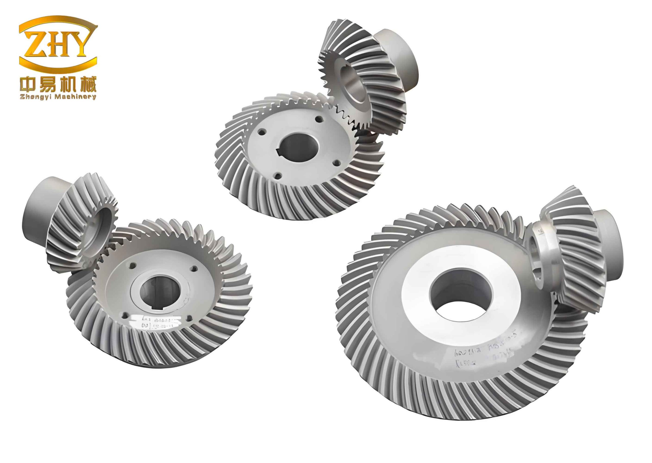
To begin, let’s consider the basic geometry of hyperboloidal gears. These gears are characterized by their skew axes, with an offset distance E and a shaft angle Σ. The design process starts with initial conditions, including the gear ratio (or tooth numbers z1 and z2), Σ, E, the gear’s outer pitch diameter D2, face width b, nominal spiral angle β10 at the pinion node, and cutter radius r0. The Gleason method estimates the gear pitch cone angle δ2′ using an approximate formula: $$ \tan \delta_2′ = \frac{z_2 \sin \Sigma}{1.2(z_1 + z_2 \cos \Sigma)} $$. This initial value, however, often leads to discrepancies, as the actual node position on the gear may not align with the face width midpoint. The gear pitch radius r2 is derived from: $$ r_2 = 0.5(D_2 – b \sin \delta_2) $$, where δ2 is refined iteratively. This iterative process is crucial for hyperboloidal gears, as it affects subsequent parameter calculations like offset angles and spiral angles.
In the Gleason approach, the calculation proceeds through several layers. First, the offset angle γ′ is determined: $$ \sin \gamma’ = \frac{E \sin \delta_2′}{r_2} $$. Then, an amplification factor k is introduced: $$ k = \cos \gamma’ + \tan \beta_{10} \sin \gamma’ $$, which helps estimate the pinion pitch radius r1: $$ r_1 = k \frac{z_2}{z_1} r_2 $$. The pinion offset angle β is approximated as: $$ \tan \beta = \frac{E}{r_1 + r_2 \cos \Sigma + r_2 \tan \delta_2′ \sin \Sigma} $$. These steps form the inner layer of the computation, aimed at ensuring the pinion spiral angle β1 closely matches the nominal value β10. However, due to simplifications, errors accumulate, necessitating multiple iterations. For example, the pinion spiral angle is recalculated using: $$ \tan \beta_1 = \frac{k – \cos \gamma’}{\sin \gamma’} $$, and if deviations exceed tolerances, k is adjusted: $$ k = k’ + (\tan \beta_1 – \tan \beta_{10}) \sin \gamma’ $$. This iterative correction is repeated until convergence, but it may not fully address all geometric constraints for hyperboloidal gears.
The outer layer of the Gleason method focuses on matching the cutter radius r0 with the limiting normal curvature radius r01. Parameters such as the gear pitch cone angle δ2, pinion pitch cone angle δ1, and spiral angles are computed: $$ \tan \delta_2 = \frac{\sin \gamma}{\tan \beta \sin \Sigma} – \cos \gamma \cot \Sigma $$, $$ R_1 = \frac{r_1}{\sin \delta_1} $$, $$ R_2 = \frac{r_2}{\sin \delta_2} $$, and $$ \beta_2 = \beta_1 – \gamma’ $$. The limiting pressure angle α* and curvature radius are approximated: $$ \sin \alpha^* = \frac{\sqrt{R_1^2 + R_2^2 – 2R_1R_2 \cos \Sigma}}{r_0} $$ and $$ r_{01} = \frac{R_1 \sin \alpha^*}{\cos \beta_1} $$. If |1 – r01/r0| > 0.01, the offset angle β is adjusted, and the process iterates again. This two-layer structure, while systematic, can lead to inaccuracies in hyperboloidal gears, particularly in node positioning and spiral angle fidelity.
To overcome these limitations, I propose a new geometric parameter calculation method for hyperboloidal gears. This approach introduces an additional intermediate parameter—the gear pitch cone angle adjustment coefficient kδ—to ensure the gear node remains at the face width midpoint. The initial estimate for δ2 is modified: $$ \tan \delta_2′ = \frac{z_2 \sin \Sigma}{k_\delta (z_1 + z_2 \cos \Sigma)} $$, with kδ initially set to 1.2. By incorporating this, the calculation hierarchy expands to three layers: computing to β1, to r01, and to δ2, as illustrated in Figure 2(b) of the original text. This added layer addresses the node shift issue, enhancing the practicality of hyperboloidal gear design.
Furthermore, I formulate the geometric parameter problem as a nonlinear least-squares optimization model. Instead of relying on step-by-step formulas, the equations are solved numerically using methods like Guess-Newton or Leverberg-Marquardt. The objective function minimizes the errors between computed and target parameters: $$ \min \left[ ( \beta_1 – \beta_{10} )^2 + ( r_{01} – r_0 )^2 + ( \delta_2 – \delta_2′ )^2 \right] $$, subject to constraints such as $$ \left| 1 – \frac{r_{01}}{r_0} \right| < \epsilon $$, where ε is a tolerance (e.g., 10⁻⁴). This mathematical model allows for simultaneous adjustment of variables, improving accuracy and convergence for hyperboloidal gears. The key variables include the offset angles, pitch radii, and spiral angles, all interlinked through geometric relations.
To demonstrate the efficacy of this new method, I present a computational example comparing it with the traditional Gleason approach. The table below summarizes the geometric parameters for a hyperboloidal gear pair, highlighting differences in critical values like spiral angles, pitch cone angles, and curvature radii. This comparison underscores the improvements offered by the novel method, particularly in reducing errors associated with hyperboloidal gears.
| Parameter Name | Traditional Gleason Method | New Proposed Method |
|---|---|---|
| Pinion Tooth Number (z1) | 10 | 10 |
| Gear Tooth Number (z2) | 41 | 41 |
| Face Width (b) | 31.750 mm | 31.750 mm |
| Offset Distance (E) | 38.100 mm | 38.100 mm |
| Gear Outer Pitch Diameter (D2) | 209.550 mm | 209.550 mm |
| Cutter Radius (r0) | 114.300 mm | 114.300 mm |
| Pinion Midpoint Spiral Angle (β10) | 50° | 50° |
| Gear Pitch Cone Angle Initial Value (δ2′) | 73°41′10″ | 74°49′47″ |
| Gear Offset Angle in Axial Plane (γ) | 6°2′28″ | 6°2′18″ |
| Pinion Offset Angle in Axial Plane (β) | 22°54′33″ | 22°57′47″ |
| Offset Angle in Pitch Plane (γ′) | 23°41′ | 23°42′8″ |
| Pinion Pitch Cone Angle (δ1) | 13°58′ | 13°56′32″ |
| Gear Pitch Cone Angle (δ2) | 74°48′ | 74°49′48″ |
| Gear Midpoint Spiral Angle (β2) | 26°19′ | 26°17′52″ |
| Pinion Midpoint Spiral Angle (β1) | 49°59′39″ | 50°0′0″ |
| Gear Midpoint Radius (r2) | 89.5392 mm | 89.4532 mm |
| Pinion Midpoint Radius (r1) | 30.4507 mm | 30.4096 mm |
| Limiting Pressure Angle (α*) | -8°26′2″ | -8°26′11″ |
| Corresponding Curvature Radius (r01) | 114.1049 mm | 114.3000 mm |
| Distance from Gear Midpoint to Pinion Axis | 30.2806 mm | 30.2806 mm |
| Distance from Gear Apex to Pinion Axis | 5.9543 mm | 6.0074 mm |
The table reveals that the new method achieves exact alignment for the pinion spiral angle (50°0′0″) and cutter radius (114.3000 mm), whereas the Gleason method shows minor deviations. Additionally, the gear pitch cone angle is more consistent with its initial estimate, reducing node shift to approximately 0.21 mm. This validates the effectiveness of the optimization-based approach for hyperboloidal gears. The mathematical model ensures that constraints are satisfied simultaneously, unlike the sequential iterations in traditional methods.
In-depth analysis of the new method involves deriving iterative equations for hyperboloidal gears. For instance, the relationship between offset angles and pitch radii can be expressed as a system of nonlinear equations: $$ \sin \gamma = \frac{E – r_1 \sin \beta}{r_2} $$, $$ \tan \delta_1 = \frac{\sin \beta}{\tan \gamma \sin \Sigma} – \frac{\cos \beta}{\tan \Sigma} $$, and $$ \tan \beta_1 = \frac{k – \cos \gamma’}{\sin \gamma’} $$. By solving these numerically, we can refine parameters like the amplification factor k and pitch radii. The use of optimization algorithms allows for handling complex interdependencies, which is crucial for hyperboloidal gears due to their non-linear geometry.
Moreover, I explore the impact of parameter variations on hyperboloidal gear performance. For example, changes in offset distance E or shaft angle Σ can significantly alter spiral angles and contact patterns. Through sensitivity analysis, the new method provides insights into design robustness. Equations such as $$ \frac{\partial \beta_1}{\partial E} = \frac{1}{r_1 \cos^2 \beta} $$ help quantify these effects, enabling designers to make informed decisions. This level of detail is essential for advancing hyperboloidal gear applications in industries like automotive, where efficiency and durability are paramount.
To further illustrate the calculations, I include additional formulas relevant to hyperboloidal gears. The pitch cone distances are given by: $$ R_1 = \sqrt{r_1^2 + E^2 – 2r_1E \cos \beta} $$ and $$ R_2 = \sqrt{r_2^2 + E^2 – 2r_2E \cos \gamma} $$. The spiral angles relate to the tooth geometry: $$ \cos \beta_2 = \frac{R_1 \cos \beta_1 – E}{R_2} $$. These equations form the backbone of the geometric model, and their accurate solution is facilitated by the new iterative method. By integrating them into the optimization framework, we ensure consistency across all parameters for hyperboloidal gears.
In conclusion, the research on geometric parameter calculation methods for hyperboloidal gears highlights the limitations of traditional approaches like the Gleason system. My proposed method, based on an enhanced iterative structure and optimization theory, addresses key issues such as pinion spiral angle accuracy, cutter radius matching, and gear node positioning. The inclusion of an adjustment coefficient kδ and a nonlinear least-squares model improves computational precision and practicality. As demonstrated through the example, this new approach offers superior results, making it a valuable tool for designers working with hyperboloidal gears. Future work could explore real-time applications or integration with CAD software, further advancing the field of gear design.