1. Introduction
Spiral bevel gears play a crucial role in various mechanical systems, especially in automotive, aerospace, and mining machinery. Their unique design, characterized by high ,strong load – bearing capacity, high ,and high transmission efficiency, makes them indispensable in power – transmitting applications . However, the manufacturing precision of spiral bevel gears is highly dependent on the accuracy of the machine tools used. Machine tool errors, including geometric errors, thermal errors, and servo – control errors, can significantly affect the quality of the gear tooth surface. Among these errors, geometric errors are particularly important as they are repetitive and stable, and can potentially be compensated through the numerical control system.
Sensitivity analysis is a powerful tool that helps in understanding how changes in input factors affect the output of a system. In the context of spiral bevel gear manufacturing, it can be used to determine which geometric errors of the machine tool have the most significant impact on the tooth surface deviation. This knowledge is essential for gear manufacturers as it enables them to focus on compensating for the critical geometric errors, thereby improving the overall quality of the gears.
The aim of this article is to provide a comprehensive understanding of the sensitivity analysis of machining deviation in spiral bevel gears. We will explore different sensitivity analysis methods, establish a machining deviation model for spiral bevel gears, and conduct case studies to compare the effectiveness of these methods. Additionally, we will discuss the selection principles of sensitivity analysis methods based on the characteristics of the input parameters and the model.
2. Sensitivity Analysis Methods
There are two main categories of sensitivity analysis methods: local sensitivity analysis methods and global sensitivity analysis methods. Each method has its own characteristics and is suitable for different types of models.
2.1 Local Sensitivity Analysis Method
Local sensitivity analysis is a single – factor analysis approach. It works by making a small change to one input factor at a time while keeping all other factors constant. The sensitivity coefficient is then determined based on the differential of the output result with respect to the input parameter or the change in the output result due to the change in the single input factor
The concept of local sensitivity is straightforward, and its calculation is relatively simple. This method is mainly applicable to linear models and models with weak non – linearity. The analysis process.
| Step | Action |
|---|---|
| 1 | Input the change amount of the 1st parameter. |
| 2 | Calculate the theoretical output result. |
| 3 | Calculate the actual output result. |
| 4 | Calculate the deviation value. |
| 5 | Increment the parameter index (\(i = i + 1\)). |
| 6 | If all parameters have been analyzed, output all deviation values; otherwise, go back to step 1. |
2.2 Sobol Global Sensitivity Analysis
Global sensitivity analysis methods take into account the range and distribution of all parameters and consider the mutual coupling effects among input parameters during the analysis. The Sobol method, a widely – used global sensitivity analysis method based on variance, calculates the sensitivity coefficients of input parameters by decomposing the variance of the model .
2.3 Monte Carlo Estimation
In the process of solving sensitivity coefficients using the Sobol method, multiple – integral solutions are often involved. For complex models, these multiple – integral solutions are usually difficult to obtain. Therefore, the Monte Carlo method is commonly used to approximate the multiple – integral solutions.
The general calculation process is as follows: two independent samplings are performed on the input parameters to obtain two independent sampling matrix results E and F. Then, based on E and F, matrices \(E_{F}^{i}\) (\(i = 1,2,\cdots,n\)) are constructed. The first – order sensitivity coefficient \(S_{i}\) and the global sensitivity coefficient \(S_{i}^{tot}\) can be approximated by the following formulas.
3. Machining Model of Spiral Bevel Gear Machine Tools
3.1 Classification of Machine Tool Geometric Errors
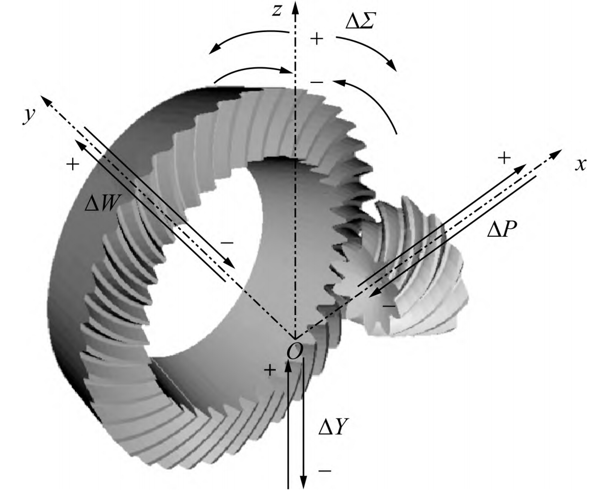
The structure of a numerical control machine tool for spiral bevel gears is shown in Figure 2. The A, B, X, Y, and Z axes work together to machine Gleason – type spiral bevel gears according to the set numerical control program. The C – axis drives the cutter head to rotate without affecting the tooth surface generation process. The coordinate transformation relationship of the machine tool is shown.
For the five motion axes related to the tooth surface generation, each axis may have geometric errors due to manufacturing and assembly factors. These geometric errors directly cause tooth surface deviations. Each axis has six geometric errors, including three linear errors and three angular errors. In total, 30 geometric errors need to be considered for the entire machine tool .
To facilitate analysis, the geometric errors are numbered as shown in Table 1.
| Coordinate Axis | Geometric Errors | Serial Number | |||||
|---|---|---|---|---|---|---|---|
| X | \(\delta_{xX}\) | \(\delta_{yX}\) | \(\delta_{zX}\) | – | – | – | 1 – 3 |
| Y | \(\delta_{xY}\) | \(\delta_{yY}\) | \(\delta_{zY}\) | – | – | – | 4 – 6 |
| Z | \(\delta_{xZ}\) | \(\delta_{yZ}\) | \(\delta_{zZ}\) | – | – | – | 7 – 9 |
| A | \(\delta_{xA}\) | \(\delta_{yA}\) | \(\delta_{zA}\) | – | – | – | 10 – 12 |
| B | \(\delta_{xB}\) | \(\delta_{yB}\) | \(\delta_{zB}\) | – | – | – | 13 – 15 |
| X | \(\varepsilon_{\alpha X}\) | \(\varepsilon_{\beta X}\) | \(\varepsilon_{\gamma X}\) | – | – | – | 16 – 18 |
| Y | \(\varepsilon_{\alpha Y}\) | \(\varepsilon_{\beta Y}\) | \(\varepsilon_{\gamma Y}\) | – | – | – | 19 – 21 |
| Z | \(\varepsilon_{\alpha Z}\) | \(\varepsilon_{\beta Z}\) | \(\varepsilon_{\gamma Z}\) | – | – | – | 22 – 24 |
| A | \(\varepsilon_{\alpha A}\) | \(\varepsilon_{\beta A}\) | \(\varepsilon_{\gamma A}\) | – | – | – | 25 – 27 |
| B | \(\varepsilon_{\alpha B}\) | \(\varepsilon_{\beta B}\) | \(\varepsilon_{\gamma B}\) | – | – | – | 28 – 30 |
3.2 Tooth Surface Machining Process
The generation motion of the workpiece gear is determined by the X, Y, Z, A, and B axes. The homogeneous transformation matrix from the A – axis to the Y – axis, when combined with the tool equation, can obtain the ideal tooth surface equation \(r_{s}\) [14]: \(r_{E}=M_{A}\cdot M_{B}\cdot M_{Z}\cdot M_{X}\cdot M_{Y}\cdot r_{t}(u,\theta)\) where \(M_{q}\) (\(q = X,Y,Z,A,B\)) is the motion transformation matrix corresponding to each axis, and \(r_{t}(u,\theta)\) is an expression obtained from the tool equation. u and \(\theta\) are cutter head parameters.
When considering the geometric errors of the machine tool, the actual tooth surface equation is: \(\begin{aligned}r_{g}^{e}&=M_{A}\cdot M_{A}^{e}\cdot M_{B}\cdot M_{B}^{e}\cdot M_{Z}\cdot M_{Z}^{e}\cdot M_{x}\cdot M_{x}^{e}\cdot\\&M_{Y}\cdot M_{Y}^{e}\cdot r_{1}(u,\theta)\end{aligned}\) where \(M_{q}^{e}\) (\(q = X,Y,Z,A,B\)) is the geometric error matrix corresponding to each axis.
4. Case Studies of Sensitivity Analysis
4.1 Sampling Calculation
We take a gear with the parameters shown in Table 2 as an example.
| Parameter | Value |
|---|---|
| Number of Teeth \(Z_{1}\) | 18 |
| Large – End Module \(m_{t}\) /mm | 4.29 |
| Tooth Face Width \(w_{b}\) /mm | 45 |
| Helical Direction | Left – Hand |
| Mid – Point Helix Angle \(\beta\) /(°) | 35 |
| Addendum \(h_{a}\) /mm | 8.78 |
| Dedendum \(h_{f}\) /mm | 5.03 |
| Pitch Cone Angle \(\gamma_{1}\) /(°) | 27.21 |
| Face Cone Angle \(\gamma_{p}\) /(°) | 31.65 |
| Root Cone Angle \(\gamma_{f}\) /(°) | 25.36 |
| Outer Cone Distance \(L_{o}\) /mm | – |
Table 2: Geometric and Machining Parameters of the Gear
Based on the equations (13) and (14), we can obtain the theoretical and actual tooth surfaces of the spiral bevel gear. To simplify the analysis, a \(15\times9\) discrete dot matrix is used to represent the tooth surface. By comparing the coordinates of the corresponding points in the theoretical and actual tooth surface dot matrices, the deviation value \(K_{f}\) of each tooth surface point can be calculated. The tooth surface deviation K, which is used to measure the overall deviation of the tooth surface, is calculated as: \(K=\sum_{j = 1}^{155}|K_{f}|\)
For local sensitivity analysis, a change of +0.01mm is given to each linear parameter, and a certain change (not specified in the original but assumed for consistency) is given to each angular parameter. The results of the local sensitivity analysis are shown.
For the Sobol global sensitivity analysis, referring to the input parameter changes in the local sensitivity analysis, the linear error range is set, and the angular error range is set to \(0^{\prime\prime}\sim27^{\prime\prime}\), with geometric error parameters following a uniform distribution. A sampling program is written to randomly sample the geometric error parameters within the given range. Then, the corresponding theoretical and actual tooth surfaces are calculated, and the tooth surface deviation K is obtained. The global sensitivity coefficients of the 30 geometric errors of the machine tool are calculated using the Sobol method, and the results are shown.
4.2 Discussion on Input Parameter Conditions
When using the local sensitivity analysis method, it is necessary to ensure that the change amounts of the same – type input parameters are the same so that the output results are comparable. The selection of this standard is independent of the actual range and distribution law of the input parameters. Therefore, changes in the actual input parameter range do not affect the local sensitivity analysis results.
In the global sensitivity analysis method, the input parameter range is usually selected with reference to the local sensitivity analysis method to ensure the same range and distribution law for the same – type parameters. However, in real – world situations, the value ranges of input parameters are often different, and their change laws also vary. Taking the geometric error with serial number 4 as an example, when its value interval is changed from \(0\sim10\mu m\) to \(0\sim20\mu m\) while keeping other conditions unchanged, the sensitivity analysis results are shown.
It can be observed that for the global sensitivity analysis method, when the input parameter value range changes, the sensitivity analysis results change significantly. For example, the global sensitivity coefficient of the geometric error item \(\delta_{sr}\) (serial number 4) increases from 0.023 to 0.154, while the global sensitivity coefficients of other items change slightly, and the relative proportions remain approximately the same.
4.3 Result Analysis
By comparing the calculation results of the two sensitivity analysis methods before and after the change of the input parameter range, the following characteristics can be found for the spiral bevel gear tooth surface machining deviation calculation model:
- Linear Error Sensitivity Coefficient Distribution: Under the ideal condition where the input parameter value range and distribution law are exactly the same, the distribution laws of the sensitivity coefficients of linear errors on the spiral bevel gear tooth surface deviation obtained by the two sensitivity analysis methods are the same. The sensitivity coefficients of the linear error terms of each axis show the order: y – direction (geometric errors with serial numbers 2, 5, 8, 11, 14) > x – direction (geometric errors with serial numbers 1, 4, 7, 10, 13) > z – direction (geometric errors with serial numbers 3, 6, 9, 12, 15).
- Angular Error Sensitivity Coefficient Distribution: Under the same ideal condition, although there are small differences in the distribution laws of the sensitivity coefficients of each axis’ angular errors on the spiral bevel gear tooth surface deviation obtained by the two sensitivity analysis methods due to the different probability calculation formulas and sampling sample limitations, the overall trends are the same. The key angular errors of each axis are the same (geometric errors with serial numbers 17, 18, 19, 20, 23, 26, 29).