Spiral bevel gears have the characteristics of high overlap, strong load-bearing capacity, high transmission ratio, and high transmission efficiency, and are widely used in fields such as automobiles, aviation, and mining machinery. The manufacturing accuracy of spiral bevel gears is directly related to the error of CNC machine tools. The errors of CNC machine tools include geometric errors, thermal errors, and servo control errors. Among them, the geometric errors of machine tools have the characteristics of repetition and stability, and can be accurately compensated through CNC systems. Therefore, studying the characteristics of geometric errors in machine tools and determining key geometric error terms plays an important role in compensating tooth surface deviations and allocating and maintaining machine tool motion accuracy.
Sensitivity analysis is an analytical method that studies the degree to which changes in input factors in a system affect output results. The analysis results are represented by sensitivity coefficients. A higher sensitivity coefficient indicates a higher correlation between the input factor and the output result. Sensitivity analysis is an important method for studying the relationship between geometric errors of machine tools and machining accuracy. In terms of sensitivity analysis of geometric errors in machine tools, scholars at home and abroad have conducted in-depth research.
CHEN et al. calculated the sensitivity coefficients of 37 geometric error terms of the machine tool using matrix differentiation method; CHENG et al. conducted sensitivity analysis on 18 geometric errors of vertical machining centers using the Sobol method; Xia Changchang et al. used the Morris method to analyze the key geometric error terms that affect the accuracy of the five axis CNC gear grinding machine; Yu Wenli et al. used the extended Fourier amplitude test method to identify strongly coupled geometric error terms and key geometric error terms. At present, although there are many sensitivity analysis methods, due to the complexity of the tooth surface of spiral bevel gears, there are many factors that affect the machining accuracy of the tooth surface. Therefore, selecting a reasonable sensitivity analysis method is crucial for sensitivity analysis of tooth surface deviation.
ZHY Gear first compares the computational principles and characteristics of local sensitivity and global sensitivity methods; Then, combining the principles of CNC machining of spiral bevel gears and sensitivity analysis methods, the sensitivity relationship between machine tool geometric errors and spiral bevel gear tooth surface deviations is studied; Finally, by analyzing the characteristics of the two sensitivity analysis methods through examples, theoretical guidance is provided for the selection of sensitivity analysis methods for the tooth surface deviation of spiral bevel gears.
1. Sensitivity analysis
There are two main types of sensitivity analysis methods: local sensitivity analysis methods represented by differential, difference, and perturbation methods, and global sensitivity analysis methods represented by regression analysis, variance, and screening methods. Through sensitivity analysis, key input factors and non key input factors can be identified. In actual analysis and calculation, non critical input factors can be ignored first, which can significantly reduce the complexity and analysis difficulty of the system, while significantly reducing the computational workload and processing difficulty of related data.
1. 1 Local sensitivity analysis method
Local sensitivity analysis is a type of single factor analysis method that determines the sensitivity coefficient by making small changes to a single input factor each time, while keeping all other factors unchanged, in order to differentiate the output results from the input parameters or the changes in the output results caused by a single input factor change. The concept of local sensitivity is clear, the calculation is simple, and it is mainly suitable for linear models and models with weak nonlinearity.
1. 2 Sobol Global Sensitivity Analysis
The global sensitivity analysis method not only considers the range and distribution pattern of each parameter, but also substitutes all parameters for analysis during the analysis and calculation process, taking into account the influence of mutual coupling between input parameters on the results. However, global sensitivity analysis methods generally require a certain scale of sampling to obtain the input parameters of the model, and then perform sensitivity analysis, especially for cases with a large number of parameters, the computational workload will be relatively large.
Taking the Sobol method as an example, it is a variance based global sensitivity method that mainly calculates the sensitivity coefficient of input parameters by decomposing the sub item variance of the model.
The number of input parameters for the model is represented by n, and the i-th input parameter is represented by xi, where i=(1, 2,…, n). Use K=f (X) to represent the multivariate function corresponding to the model, where X=(x1, x2,…, xn). The decomposition of f (X) is as follows:

In the formula: f0 is the expected value of the output result f (X) calculated from the input parameters, which is a constant; Fi (xi) represents the output result under the independent action of the input parameter xi; Fi, j (xi, xj) represents the output result under the joint action of input parameters xi and xj; F1,…, n (x1, x2,…, xn) represents the output result under the joint action of all input parameters; The other orders can be obtained similarly.
The total variance D can be expressed in the following form:

The variance components can be obtained as follows:

In the formula: 1 ≤ s ≤ n.
Using the Sobol method, the left and right sides of equation (1) are first squared and then integrated to obtain:

The sensitivity coefficient can be obtained by the following formula:
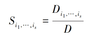
Because the variance is non negative, it is known that Si1,…, is are non negative numbers. According to equations (4) and (5), we can obtain:

In the formula, Si is the first-order sensitivity coefficient corresponding to the variable xi; Si, j (i<j) is the second-order sensitivity coefficient corresponding to the coupling effect between variables xi and xj. Similarly, sensitivity coefficients for each order can be obtained. The global sensitivity coefficient Stoti corresponding to variable xi can be obtained by summing up the sensitivity coefficients related to variable xi. The calculation method is as follows:

In the formula, the range of values for the positive integer k is: 1 ≤ k ≤ n, and k ≠ i.
1.3 Monte Carlo estimation
The use of Sobol method in solving sensitivity coefficients involves multiple integration solutions, which are often very difficult for complex models. Therefore, Monte Carlo method is often used to approximate multiple integration solutions. The general calculation method is as follows: perform two independent samplings on the input parameters to obtain two independent sampling matrices, E and F. The results are as follows:
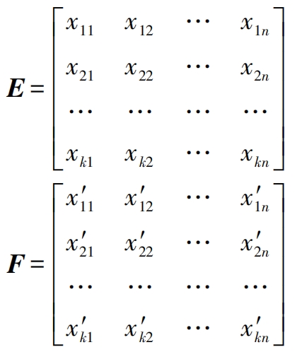
In the formula, k represents the number of spiral bevel gear samples sampled each time. To solve for the first-order sensitivity coefficient and global sensitivity coefficient, a matrix EiF is constructed based on two matrices E and F, where i=1, 2,…, n. Matrix EiF is obtained by replacing the i-th column with the i-th column of matrix F based on matrix E. The rest of the matrix is identical to matrix E. Matrix EiF can be expressed in the following form:
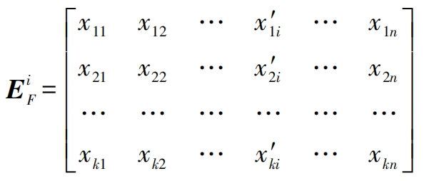
A row of the spiral bevel gear sample matrix represents a complete set of input parameter spiral bevel gear samples. Therefore, the input parameters of each row can be solved separately to obtain a model output result. The first-order sensitivity coefficient Si and the global sensitivity coefficient Stud can be approximately calculated using the following formula:
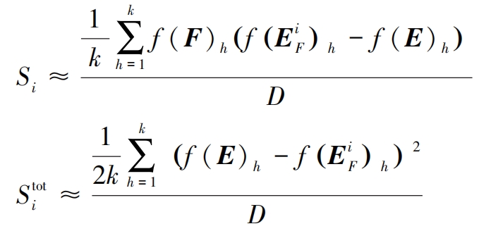
In the formula: f (E) h is the output result obtained by substituting the h-th row of matrix E into the model; F (F) h is the output result obtained by substituting the h-th row of matrix F into the model solution; F (EiF) h is the output result obtained by substituting the h-th row of the matrix EiF into the model
2. Spiral bevel gear machining model
2.1 Classification of geometric errors in machine tools
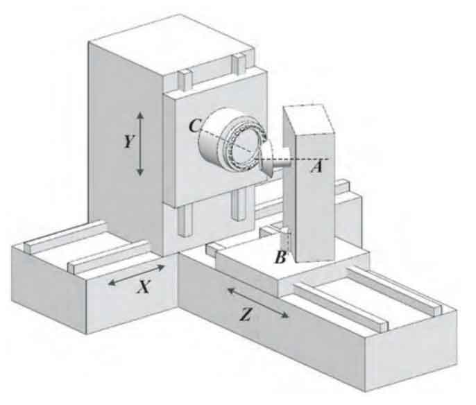
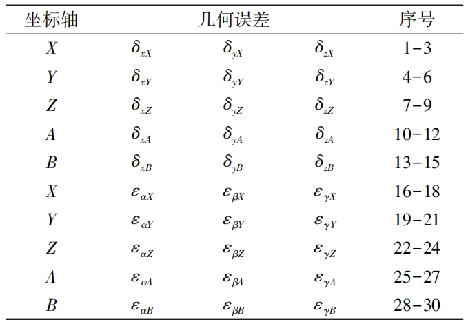
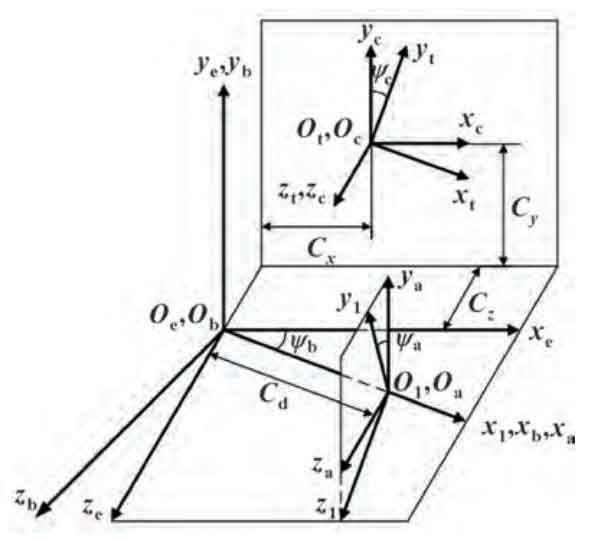
The structure of the CNC machine tool is shown in Figure 1: according to the set CNC program, the A, B, X, Y, and Z axes are linked, and the Gleason spiral bevel gears can be machined. The C-axis drives the cutter head to rotate without affecting the tooth surface formation process. The coordinate transformation relationship of the machine tool is shown in Figure 2. For the 5 motion axes related to tooth surface development, each axis is affected by manufacturing, assembly, and other factors, resulting in geometric errors that directly lead to tooth surface deviations. Each axis has 6 geometric errors, including 3 linear errors and 3 angular errors. For the entire machine tool, 30 geometric errors need to be considered.
For the convenience of analysis, the geometric error sequence is numbered as shown in Table 1. Among them ε Represents angle error, δ Representing linear error, the error variable is distinguished by two subscripts: the first subscript represents the direction of the error, and the second subscript represents the axis on which the error is located. For example: εα Y represents the Y-axis in α Angle error in direction, ε YX represents the linear error of the X-axis in the y-direction.
2.2 Tooth surface machining process
The generating motion of spiral bevel gears is determined by the five axes X, Y, Z, A, and B. So the homogeneous transformation matrix from the A-axis to the Y-axis can be combined with the tool equation to obtain the ideal tooth surface equation rg.

In the formula: Mq (q=X, Y, Z, A, B) is the motion transformation matrix corresponding to each axis; Rt is an expression obtained from the tool equation; U and θ The parameters for the cutterhead. Due to limited space, the specific process can be referred to in the literature.
If considering the geometric error of the machine tool, the actual tooth surface equation is as follows:

In the formula, Meq (q=X, Y, Z, A, B) is the geometric error matrix corresponding to each axis.
3. Example of sensitivity analysis
3.1 Sampling calculation
Taking the spiral bevel gear shown in Table 2 as an example, the theoretical tooth surface of the spiral bevel gear can be obtained according to equation (13). Considering the influence of machine tool geometric errors in actual machining, the actual tooth surface of the spiral bevel gear can be calculated according to equation (14).
| Parameters | Numerical value |
| Number of teeth Z1 | 18 |
| Large end modulus mt/mm | 4.29 |
| Tooth surface width wb/mm | 45 |
| Rotation direction | Left-handed rotation |
| Midpoint helix angle β / (°) | 35 |
| Tooth top height h a/mm | 8.78 |
| Root height h f/mm | 5.03 |
| Pitch cone angle γ 1/(°) | 27.21 |
| Face cone angle γ P/(°) | 31.65 |
| Root cone angle γ F/(°) | 25.36 |
| Outer cone distance Lo/mm | 140.9 |
For the convenience of analysis and calculation, a discrete 15 × 9 lattice is used to represent the tooth surface. By combining equations (13) and (14), the theoretical tooth surface lattice and the actual tooth surface lattice can be obtained. By using the coordinate values of the corresponding points in the lattice, the deviation value Kf of the corresponding tooth surface points can be calculated, where f represents the number of points in the lattice. K represents tooth surface deviation, which is the output result of the calculation model used to measure the magnitude of tooth surface deviation. It can be obtained by the following formula:
The variation of each linear parameter is given as+0 01mm, the variation of each angle parameter is+27 inches. Using the tooth surface deviation K as the model output result, the local sensitivity analysis results are shown in Figure 3.
Referring to the input parameter variation in local sensitivity analysis, a linear error range of 0-10 is given μ m. The range of angle error is 0 “to 27”, and the geometric error parameters follow a uniform distribution. Write a sampling program to randomly sample within the given range of geometric errors and generate machine tool geometric error parameters. By combining equations (13) and (14), the corresponding theoretical tooth surface and actual tooth surface can be calculated. Based on the lattice of the two tooth surfaces, the corresponding tooth surface deviation K can be solved.
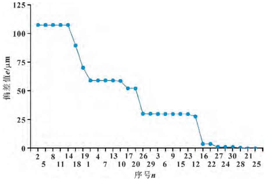
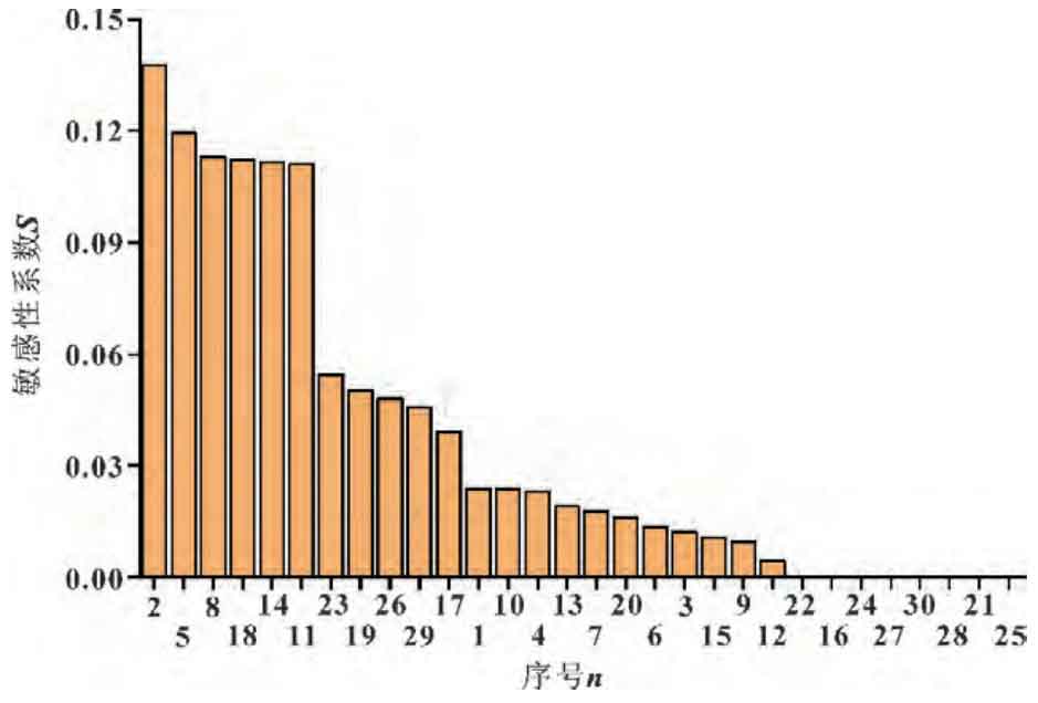
The Sobol global sensitivity analysis method can be used to solve the global sensitivity coefficients of 30 machine tool geometric errors, arranged in descending order of global sensitivity coefficients, as shown in Figure 4.
3.2 Discussion on Input Parameter Situation
The use of local sensitivity analysis methods for sensitivity analysis requires ensuring that the changes in input parameters of the same type are the same, so that the output results are comparable. The selection criteria are independent of the actual range and distribution pattern of input parameters, so changes in the actual range of input parameter values will not affect the results of local sensitivity analysis.
In the previous text, the selection of the input parameter range for the global sensitivity analysis method referred to the characteristics of the local sensitivity analysis method, ensuring that the range and distribution pattern of the same type of parameter are the same. However, in real situations, the range of input parameter values is generally different, and the variation pattern is also often different. So, considering the actual possible situation, taking the geometric error with serial number 4 as an example, let the value range of this geometric error be from 0 to 10 μ M changes from 0 to 20 μ m. Keep other conditions unchanged at the same time. The sensitivity analysis results can be obtained as shown in Figure 5.
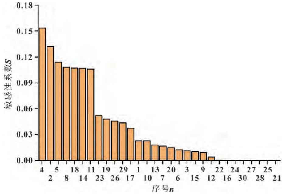
It can be observed that for the global sensitivity analysis method, after changing the range of input parameters, the results of sensitivity analysis undergo significant changes. Among them, the geometric error term with serial number 4, i.e δ XY, the global sensitivity coefficient has undergone a significant change from the original 0 023 increased to 0 154. The global sensitivity coefficients of other items only show slight changes, and there is no significant change in the relevant proportions.
3.3 Pairs of fruit scoring analysis
Comparing the calculation results of the two sensitivity analysis methods before and after the range change, it can be found that for the calculation model of machining deviation of spiral bevel gears, the two sensitivity analysis methods have the following characteristics:
(1) In the ideal situation where the range and distribution of input parameter values are exactly the same, the sensitivity coefficient distribution of the linear error obtained by the two sensitivity analysis methods to the tooth surface deviation of spiral bevel gears is the same. The sensitivity coefficients of the linear error terms for all 5 axes show a trend of y-direction (geometric errors numbered 2, 5, 8, 11, 14)>x-direction (geometric errors numbered 1, 4, 7, 10, 13)>z-direction (geometric errors numbered 3, 6, 9, 12, 15).
(2) In the ideal situation where the range and distribution of input parameter values are exactly the same, the sensitivity coefficient distribution of the angle error of each axis on the tooth surface deviation of spiral bevel gears obtained by the two sensitivity analysis methods has a small difference due to the probability calculation formula and sampling sample limitations used, but the overall trend is the same. The key angle errors of each axis are the same (geometric errors numbered 17, 18, 19, 20, 23, 26, 29).
(3) When the range of input parameter values changes, global sensitivity analysis can reveal that input parameters that were originally non critical geometric errors may change to critical geometric errors. However, for local sensitivity analysis methods, their analysis results are independent of the distribution range of input parameters. When there is a significant difference in the distribution range of input parameters, the accuracy of the analysis results of this method will significantly decrease, and may no longer be suitable for sensitivity analysis of the model.
4. Conclusion
By applying two sensitivity analysis methods to the sensitivity analysis of the machining deviation model of spiral bevel gears, it can be found that:
(1) In the ideal situation where the range and distribution pattern of input parameter values are exactly the same, the local sensitivity analysis method has a smaller computational cost and can quickly obtain preliminary analysis results. At the same time, the distribution pattern of this analysis result is the same as that of the global sensitivity analysis result, which has certain reference value.
(2) The Sobol global sensitivity analysis method considers the influence of input parameter values and distribution patterns on the analysis results, making it more scientific, obtaining more credible conclusions, and having a wider range of applications. In addition, most global sensitivity analyses can be used to study the quantitative relationship between input parameters and output results, as well as the impact of parameter interactions on output results. However, compared to local sensitivity analysis methods, the computational complexity significantly increases and requires more time.
(3) For models with unclear distribution range of input parameters, limited available time, and similar or similar linear or non-linear distributions, local sensitivity analysis can be considered; For nonlinear models with complex distribution ranges and high accuracy requirements of input parameters, global sensitivity analysis methods can be considered.
ZHY Gear’s research provides theoretical guidance for the use of sensitivity analysis methods in spiral bevel gear tooth surface machining, providing reference for the selection of sensitivity analysis methods.
