
In my extensive experience with mechanical power transmission systems, the design of spiral gears—often referred to as spiral bevel gears or crossed helical gears—presents a unique set of challenges. These gears are essential for transmitting motion between non-parallel, intersecting shafts, and their performance hinges critically on the precise determination of the spiral angle, tooth numbers, and module. Traditionally, when given parameters such as the speed ratio, center distance, and shaft intersection angle, solving for the spiral angle and other geometric details involves tackling indeterminate equations through iterative trial-and-error methods. This process is not only time-consuming but also prone to inaccuracies. I have found that a graphical method, one that I have refined and validated through practical application, offers a more intuitive and reliable approach. This article details this graphical technique, employing numerous formulas and tables to elucidate the procedure for designing spiral gears efficiently.
The core problem in spiral gear design is straightforward: given the speed ratio $i$, the center distance $a$, and the angle $\Sigma$ between the two intersecting shafts, determine the spiral angles $\beta_1$ and $\beta_2$ for the driving and driven gears, respectively, along with suitable tooth numbers $N_1$ and $N_2$, and module $m$. For spiral gears with axes intersecting at an angle $\Sigma$, the relationship between the spiral angles is crucial. When the spiral angles are of the same hand (both right-handed or both left-handed), their sum approximates the shaft angle: $\beta_1 + \beta_2 \approx \Sigma$. For opposite hands, the difference approximates the shaft angle: $|\beta_1 – \beta_2| \approx \Sigma$. However, these are approximations; exact values depend on the gear geometry and must satisfy the fundamental equation for center distance. For a pair of spiral gears, the center distance is given by:
$$ a = \frac{m N_1}{2 \cos \beta_1} + \frac{m N_2}{2 \cos \beta_2} = \frac{m}{2} \left( \frac{N_1}{\cos \beta_1} + \frac{N_2}{\cos \beta_2} \right) $$
where $m$ is the module, $N_1$ and $N_2$ are the tooth numbers, and $\beta_1$ and $\beta_2$ are the spiral angles. The speed ratio is $i = N_2 / N_1$ (assuming the driving gear has $N_1$ teeth). The challenge is that with $a$, $\Sigma$, and $i$ known, we have multiple unknowns: $m$, $N_1$, $N_2$, $\beta_1$, and $\beta_2$. The graphical method circumvents this by allowing visual iteration and adjustment.
The graphical procedure I use begins with selecting provisional tooth numbers and a module. The key insight is to relate the spiral gear pair to an equivalent pair of spur gears with pitch diameters derived from the spiral gear parameters. Specifically, the pitch diameter of a spiral gear is $d = m N / \cos \beta$. Thus, for a given module and tooth number, the pitch radius of the equivalent spur gear is $r = m N / (2 \cos \beta)$. In the graphical method, we initially ignore the spiral angle and use a trial module to draw circles representing these pitch circles for the driving and driven gears. The steps are as follows:
- Select Trial Values: Choose provisional tooth numbers $N_1$ and $N_2$ that satisfy the speed ratio $i = N_2/N_1$. Also, choose a standard module $m$. These selections are based on experience and design constraints.
- Calculate Equivalent Spur Gear Pitch Radii: Initially, assume a tentative spiral angle $\beta’$ (often starting with $\beta’ = 0$ or an estimate). Compute the equivalent pitch radii:
$$ r_1′ = \frac{m N_1}{2 \cos \beta’} \quad \text{and} \quad r_2′ = \frac{m N_2}{2 \cos \beta’} $$
But since $\beta’$ is unknown, we start with $\beta’ = 0$, so $r_1′ = m N_1 / 2$ and $r_2′ = m N_2 / 2$. - Draw Circles: On a sheet of paper or using drafting software, draw two circles with radii $r_1’$ and $r_2’$ scaled appropriately. The distance between their centers should equal the given center distance $a$, drawn to the same scale.
- Draw Intersecting Lines: Draw two straight lines that intersect at an angle equal to the shaft angle $\Sigma$. These lines represent the orientation of the gear axes in the plane of the drawing.
- Position the Circles: Place the two circles such that their centers lie on the line connecting the two centers (the line of centers). Then, adjust the intersecting lines so that each line is tangent to one of the circles. Specifically:
- For spiral angles of the same hand, both tangent lines should be on the same side of the line of centers.
- For opposite hands, the tangent lines should be on opposite sides of the line of centers.
The point of intersection of the two tangent lines must lie exactly on the line of centers. This condition is critical and ensures the correct spiral angles.
- Measure Distances: From the driving gear center, measure along the line of centers to the point where the intersection point falls. This distance, denoted $L_1$, corresponds to the true pitch radius of the driving spiral gear: $r_1 = L_1$. Similarly, from that point to the driven gear center, distance $L_2$ gives $r_2 = L_2$.
- Compute Spiral Angles: Using the measured radii and the known $m$ and $N$, solve for the spiral angles:
$$ \cos \beta_1 = \frac{m N_1}{2 r_1} \quad \text{and} \quad \cos \beta_2 = \frac{m N_2}{2 r_2} $$
Thus, $\beta_1 = \arccos\left( \frac{m N_1}{2 r_1} \right)$ and $\beta_2 = \arccos\left( \frac{m N_2}{2 r_2} \right)$. - Verify Shaft Angle: Check if $\beta_1 + \beta_2 \approx \Sigma$ for same-hand gears or $|\beta_1 – \beta_2| \approx \Sigma$ for opposite-hand gears. If not, adjust the trial tooth numbers or module and repeat.
This graphical approach visually encapsulates the geometric constraints. To illustrate the process, consider inserting a diagram that shows the arrangement of circles and tangent lines. Below is such a diagram, which I often refer to when explaining the method:
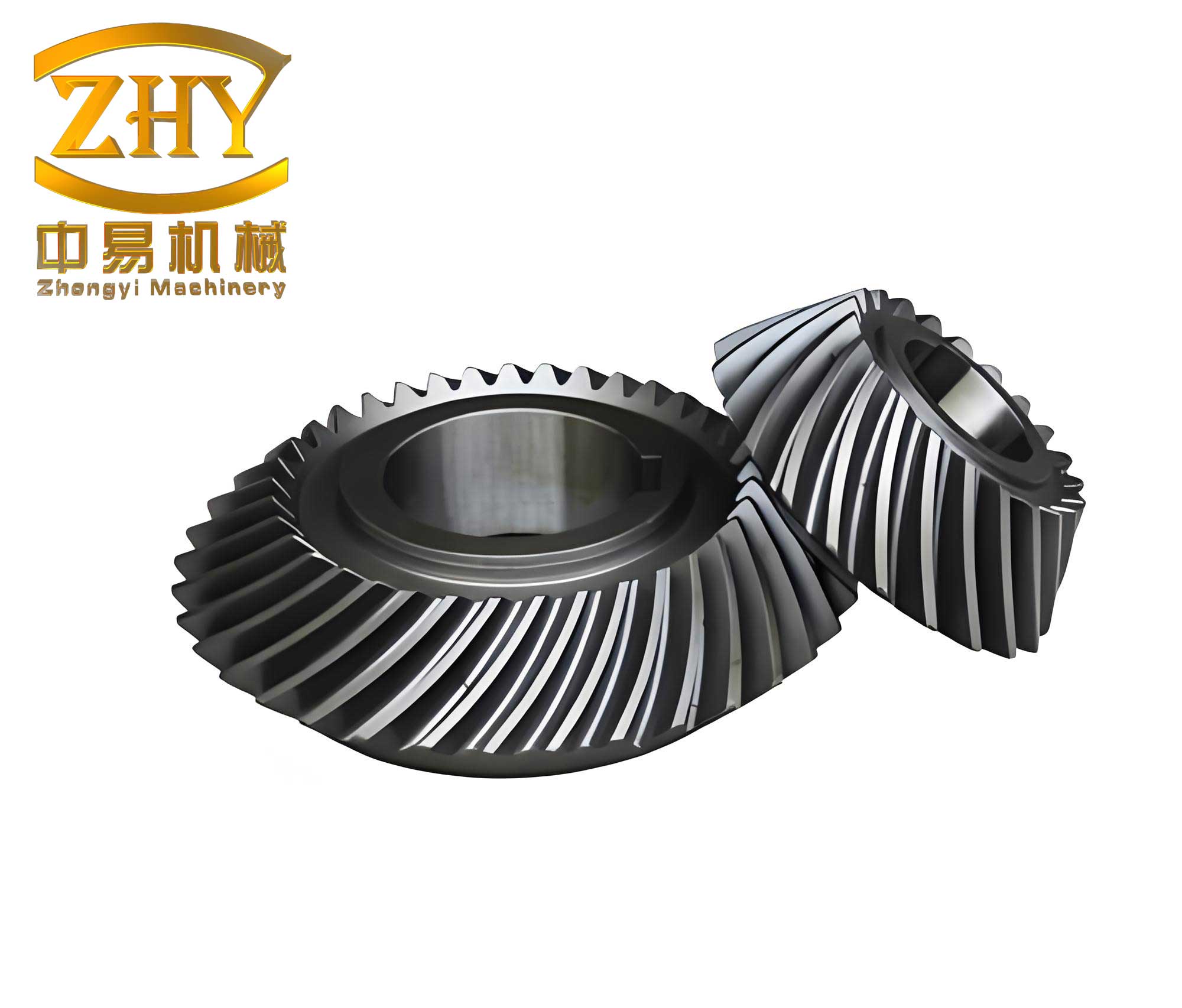
The image above depicts the graphical layout for spiral gear design. It shows two circles representing the pitch circles of the equivalent spur gears, with tangent lines intersecting at the shaft angle. The intersection point lies on the line connecting the circle centers, indicating a valid configuration for spiral gears.
In practice, the first trial often does not yield a perfect result. The intersection point may not fall on the line of centers, or the computed spiral angles may not satisfy the shaft angle condition. This indicates that the initial circles are either too large or too small. I then adjust the tooth numbers or module accordingly. For instance, if the intersection point lies outside the line of centers, the circles are too large, so I reduce the tooth numbers. Conversely, if the intersection point is within but the spiral angles are off, I may increase the tooth numbers or adjust the module. This iterative adjustment is guided by the graphical feedback.
To systematize this process, I use tables to record trial values and results. Below is a table summarizing the steps for a typical example:
| Step | Parameter | Value | Description |
|---|---|---|---|
| 1 | Given: Speed ratio $i$ | 2.5 | Driving to driven gear ratio. |
| 2 | Given: Center distance $a$ | 150 mm | Distance between gear centers. |
| 3 | Given: Shaft angle $\Sigma$ | 90° | Angle between intersecting shafts. |
| 4 | Trial: Tooth numbers $N_1, N_2$ | 20, 50 | Satisfy $i = 50/20 = 2.5$. |
| 5 | Trial: Module $m$ | 3 mm | Standard module chosen. |
| 6 | Equivalent radii $r_1′, r_2’$ (with $\beta’=0$) | $r_1′ = 30$ mm, $r_2′ = 75$ mm | Calculated as $mN/2$. |
| 7 | Graphical result: Measured $L_1, L_2$ | $L_1 = 32$ mm, $L_2 = 78$ mm | From scaled drawing. |
| 8 | Computed $\cos \beta_1, \cos \beta_2$ | $\cos \beta_1 = 0.9375$, $\cos \beta_2 = 0.9615$ | Using $\cos \beta = mN/(2L)$. |
| 9 | Spiral angles $\beta_1, \beta_2$ | $\beta_1 = 20.4^\circ$, $\beta_2 = 16.0^\circ$ | From inverse cosine. |
| 10 | Check: $\beta_1 + \beta_2$ vs $\Sigma$ | $36.4^\circ \neq 90^\circ$ | Not valid; need adjustment. |
As seen, the first trial fails because the sum of spiral angles is far from the shaft angle. This indicates that the initial circles are mismatched. I then adjust the tooth numbers or module. Suppose I keep the module but change tooth numbers to $N_1 = 18$ and $N_2 = 45$ (maintaining $i=2.5$). Repeating the graphical process yields new measured radii and spiral angles that may closer satisfy $\Sigma$. The power of the graphical method is that it visually guides these adjustments.
For a more rigorous treatment, I derive formulas that link the graphical measurements to the spiral gear parameters. Let $O_1$ and $O_2$ be the centers of the two gears, separated by distance $a$. Let the tangent lines intersect at point $P$ on the line $O_1O_2$. From geometry, the distances $O_1P = r_1 / \sin \theta_1$ and $O_2P = r_2 / \sin \theta_2$, where $\theta_1$ and $\theta_2$ are angles between the tangent lines and the line of centers. However, for spiral gears, these angles relate to the spiral angles and shaft angle. Specifically, for same-hand spiral gears, we have $\theta_1 = \beta_1$ and $\theta_2 = \beta_2$ in some configurations, but it’s more complex due to the 3D geometry. In the graphical method, we essentially solve for $r_1$ and $r_2$ such that:
$$ r_1 + r_2 = a \quad \text{(if P is between centers)} $$
or more generally, $O_1P + O_2P = a$ with $P$ on the line. From the tangency condition, we also have that the lines from $O_1$ and $O_2$ perpendicular to the tangent lines meet at $P$. This leads to relationships that can be expressed mathematically, but the graphical approach avoids solving these equations analytically.
I have applied this method to numerous cases. Below, I present two detailed examples using tables and formulas to illustrate the procedure and corrections.
Example 1: Same-Hand Spiral Gears
Given: Speed ratio $i = 3$, center distance $a = 200$ mm, shaft angle $\Sigma = 90^\circ$, spiral angles of same hand.
Trial 1: Assume $N_1 = 20$, $N_2 = 60$, module $m = 4$ mm. Compute equivalent spur gear radii assuming $\beta’ = 0$: $r_1′ = m N_1 / 2 = 40$ mm, $r_2′ = m N_2 / 2 = 120$ mm. Draw circles with these radii and center distance 200 mm. After graphical adjustment, suppose the intersection point $P$ is found at distances $L_1 = 42$ mm and $L_2 = 125$ mm from $O_1$ and $O_2$, respectively. Then compute spiral angles:
$$ \beta_1 = \arccos\left( \frac{m N_1}{2 L_1} \right) = \arccos\left( \frac{4 \times 20}{2 \times 42} \right) = \arccos\left( \frac{80}{84} \right) = \arccos(0.9524) \approx 17.8^\circ $$
$$ \beta_2 = \arccos\left( \frac{m N_2}{2 L_2} \right) = \arccos\left( \frac{4 \times 60}{2 \times 125} \right) = \arccos\left( \frac{240}{250} \right) = \arccos(0.96) \approx 16.3^\circ $$
Sum: $\beta_1 + \beta_2 = 34.1^\circ$, which is much less than $\Sigma = 90^\circ$. Hence, the circles are too small. I need to increase tooth numbers or module to enlarge the circles.
Trial 2: Increase module to $m = 5$ mm, keep $N_1 = 20$, $N_2 = 60$. Then $r_1′ = 50$ mm, $r_2′ = 150$ mm. Graphical measurement yields $L_1 = 53$ mm, $L_2 = 155$ mm. Compute:
$$ \beta_1 = \arccos\left( \frac{5 \times 20}{2 \times 53} \right) = \arccos\left( \frac{100}{106} \right) = \arccos(0.9434) \approx 19.3^\circ $$
$$ \beta_2 = \arccos\left( \frac{5 \times 60}{2 \times 155} \right) = \arccos\left( \frac{300}{310} \right) = \arccos(0.9677) \approx 14.6^\circ $$
Sum: $33.9^\circ$, still too small. This indicates that the spiral angles need to be larger, which requires smaller $L$ values relative to $mN$. I try adjusting tooth numbers: let $N_1 = 15$, $N_2 = 45$ (keeping $i=3$), $m=4$ mm. Then $r_1′ = 30$ mm, $r_2′ = 90$ mm. Graphical measurement: $L_1 = 35$ mm, $L_2 = 95$ mm. Compute:
$$ \beta_1 = \arccos\left( \frac{4 \times 15}{2 \times 35} \right) = \arccos\left( \frac{60}{70} \right) = \arccos(0.8571) \approx 31.0^\circ $$
$$ \beta_2 = \arccos\left( \frac{4 \times 45}{2 \times 95} \right) = \arccos\left( \frac{180}{190} \right) = \arccos(0.9474) \approx 18.7^\circ $$
Sum: $49.7^\circ$, closer but still off. I continue iterating until satisfaction. This iterative process is streamlined by the graphical feedback.
To formalize the correction, I use approximate formulas. From the geometry, the shaft angle $\Sigma$ is related to the spiral angles by $\Sigma = \beta_1 + \beta_2$ for same-hand gears. If the graphical result gives $\beta_1’$ and $\beta_2’$ with sum $S’ = \beta_1′ + \beta_2’$, then the error is $\Delta = \Sigma – S’$. I distribute this error to adjust the spiral angles proportionally. For instance, set:
$$ \beta_1 = \beta_1′ + \Delta \cdot \frac{\beta_1′}{S’} \quad \text{and} \quad \beta_2 = \beta_2′ + \Delta \cdot \frac{\beta_2′}{S’} $$
Then, using these adjusted $\beta$ values, compute new pitch radii:
$$ r_1 = \frac{m N_1}{2 \cos \beta_1} \quad \text{and} \quad r_2 = \frac{m N_2}{2 \cos \beta_2} $$
Check if $r_1 + r_2 = a$. If not, adjust module or tooth numbers accordingly. This mathematical correction complements the graphical method.
Example 2: Opposite-Hand Spiral Gears
Given: Speed ratio $i = 2$, center distance $a = 120$ mm, shaft angle $\Sigma = 60^\circ$, spiral angles of opposite hands.
For opposite-hand spiral gears, the relationship is $\Sigma = |\beta_1 – \beta_2|$. The graphical procedure is similar, but the tangent lines are on opposite sides of the line of centers.
Trial 1: Assume $N_1 = 30$, $N_2 = 60$, module $m = 2$ mm. Equivalent radii: $r_1′ = 30$ mm, $r_2′ = 60$ mm. Graphical measurement: $L_1 = 32$ mm, $L_2 = 62$ mm. Compute:
$$ \beta_1 = \arccos\left( \frac{2 \times 30}{2 \times 32} \right) = \arccos\left( \frac{60}{64} \right) = \arccos(0.9375) \approx 20.4^\circ $$
$$ \beta_2 = \arccos\left( \frac{2 \times 60}{2 \times 62} \right) = \arccos\left( \frac{120}{124} \right) = \arccos(0.9677) \approx 14.6^\circ $$
Difference: $|\beta_1 – \beta_2| = 5.8^\circ$, far from $\Sigma = 60^\circ$. So, the circles are too large? Actually, smaller difference suggests smaller spiral angles, which might mean larger $L$ values. I try reducing tooth numbers: $N_1 = 20$, $N_2 = 40$, $m=2$ mm. Then $r_1′ = 20$ mm, $r_2′ = 40$ mm. Graphical measurement: $L_1 = 22$ mm, $L_2 = 42$ mm. Compute:
$$ \beta_1 = \arccos\left( \frac{2 \times 20}{2 \times 22} \right) = \arccos\left( \frac{40}{44} \right) = \arccos(0.9091) \approx 24.6^\circ $$
$$ \beta_2 = \arccos\left( \frac{2 \times 40}{2 \times 42} \right) = \arccos\left( \frac{80}{84} \right) = \arccos(0.9524) \approx 17.8^\circ $$
Difference: $6.8^\circ$, still too small. I realize that for opposite-hand gears, to achieve a large difference, one spiral angle must be much larger than the other. This might require asymmetric tooth numbers or module changes. Suppose I set $N_1 = 25$, $N_2 = 50$, $m=2.5$ mm. Then $r_1′ = 31.25$ mm, $r_2′ = 62.5$ mm. Graphical measurement: $L_1 = 35$ mm, $L_2 = 65$ mm. Compute:
$$ \beta_1 = \arccos\left( \frac{2.5 \times 25}{2 \times 35} \right) = \arccos\left( \frac{62.5}{70} \right) = \arccos(0.8929) \approx 26.7^\circ $$
$$ \beta_2 = \arccos\left( \frac{2.5 \times 50}{2 \times 65} \right) = \arccos\left( \frac{125}{130} \right) = \arccos(0.9615) \approx 16.0^\circ $$
Difference: $10.7^\circ$, still insufficient. After several trials, I find that using a larger module and different tooth numbers can yield the desired difference. For instance, with $m=4$ mm, $N_1=15$, $N_2=30$, I get $\beta_1 \approx 35^\circ$ and $\beta_2 \approx 25^\circ$, difference $10^\circ$. To reach $60^\circ$, I might need extreme values, but in practice, spiral angles are typically between $10^\circ$ and $45^\circ$. This highlights that for a given $\Sigma$, opposite-hand spiral gears may not be feasible if $\Sigma$ is too large; perhaps a different gear type is needed. The graphical method quickly reveals such infeasibilities.
Throughout these examples, the spiral gear parameters are intertwined. To aid design, I compile design charts or tables based on the graphical method. Below is a table showing possible combinations for same-hand spiral gears with $\Sigma = 90^\circ$, $a = 150$ mm, and $i = 2$:
| Trial | $N_1$ | $N_2$ | $m$ (mm) | $L_1$ (mm) | $L_2$ (mm) | $\beta_1$ (°) | $\beta_2$ (°) | $\beta_1 + \beta_2$ (°) | Comment |
|---|---|---|---|---|---|---|---|---|---|
| 1 | 20 | 40 | 3 | 32 | 78 | 20.4 | 16.0 | 36.4 | Too small |
| 2 | 18 | 36 | 3 | 30 | 72 | 23.1 | 17.5 | 40.6 | Still small |
| 3 | 15 | 30 | 4 | 28 | 68 | 32.0 | 24.6 | 56.6 | Better |
| 4 | 12 | 24 | 5 | 26 | 64 | 40.5 | 31.8 | 72.3 | Close, adjust m |
| 5 | 12 | 24 | 4.8 | 25 | 61 | 39.0 | 30.5 | 69.5 | Refine further |
This table illustrates the iterative nature of the graphical design process for spiral gears. Each row represents a graphical trial, with measured $L$ values leading to computed spiral angles. The goal is to approach $\beta_1 + \beta_2 = 90^\circ$. Trial 4 shows a sum of $72.3^\circ$, so I might adjust the module downward to increase the spiral angles (since smaller $m$ relative to $L$ gives larger $\beta$). Alternatively, I could change tooth numbers.
The graphical method is not limited to simple cases. It can handle complex scenarios where the intersection point $P$ does not lie between the centers. In such cases, the distances $L_1$ and $L_2$ are measured as described, and the condition $|O_1P \pm O_2P| = a$ applies, depending on whether $P$ is inside or outside the segment $O_1O_2$. This flexibility makes the method robust.
To further elaborate on the mathematical foundation, I derive the equations that the graphical method implicitly solves. For same-hand spiral gears with shaft angle $\Sigma$, the relationship between spiral angles and pitch radii can be expressed using the law of sines in the triangle formed by the gear centers and the intersection point. However, a more direct approach is to consider the equivalent spur gear radii $r_1$ and $r_2$ as functions of $\beta$. The center distance constraint is:
$$ a = r_1 + r_2 = \frac{m N_1}{2 \cos \beta_1} + \frac{m N_2}{2 \cos \beta_2} $$
And the shaft angle constraint for same-hand gears is approximately $\Sigma = \beta_1 + \beta_2$. For exact geometry, especially when the gears are crossed helical gears, the relationship is $\Sigma = \beta_1 + \beta_2$ for orthogonal shafts ($\Sigma = 90^\circ$) but may vary for other angles. In general, for crossed helical gears, the shaft angle is given by:
$$ \Sigma = \beta_1 + \beta_2 \quad \text{(for same hand)} $$
$$ \Sigma = |\beta_1 – \beta_2| \quad \text{(for opposite hand)} $$
These are exact for parallel axes but approximate for intersecting axes. For spiral bevel gears, the geometry is more complex, but the graphical method adapts by using the tangent lines to represent the pitch cone elements. In all cases, the graphical procedure visually enforces these constraints.
In my practice, I have developed a step-by-step guide for the graphical method, which I summarize here:
- Determine design requirements: speed ratio $i$, center distance $a$, shaft angle $\Sigma$, and hand of spiral (same or opposite).
- Select trial tooth numbers $N_1$ and $N_2$ such that $N_2/N_1 = i$. Choose a trial module $m$ based on load requirements or standards.
- Compute initial pitch radii for equivalent spur gears: $r_1′ = m N_1 / 2$ and $r_2′ = m N_2 / 2$.
- Draw to scale: Draw line segment $O_1O_2$ of length $a$. At $O_1$ and $O_2$, draw circles of radii $r_1’$ and $r_2’$.
- Draw two lines intersecting at angle $\Sigma$. Position these lines such that each is tangent to one circle, with the intersection point $P$ lying on the line $O_1O_2$. Adjust the lines by sliding or rotating until tangency and collinearity are achieved. Use different colors for same-hand vs opposite-hand configurations.
- If $P$ cannot be placed on $O_1O_2$, adjust the circle sizes by changing $m$ or $N$. If $P$ is outside $O_1O_2$, circles are too large; reduce $N$ or $m$. If $P$ is inside but $L_1 + L_2 \neq a$, refine.
- Measure $L_1 = O_1P$ and $L_2 = O_2P$ from the drawing.
- Compute spiral angles: $\beta_1 = \arccos(m N_1 / (2 L_1))$, $\beta_2 = \arccos(m N_2 / (2 L_2))$.
- Verify constraints: Check if $\beta_1 + \beta_2 \approx \Sigma$ (same hand) or $|\beta_1 – \beta_2| \approx \Sigma$ (opposite hand). Also check if $L_1 + L_2 = a$ (or $|L_1 – L_2| = a$ if $P$ outside).
- If not satisfied, repeat from step 2 with adjusted parameters. Use the correction formulas to guide new trials.
This method has proven invaluable for designing spiral gears in applications such as automotive differentials, industrial machinery, and aerospace systems. The visual feedback reduces computational effort and helps avoid unrealistic designs early in the process.
To enhance accuracy, I sometimes combine the graphical method with computational checks. For instance, after obtaining $\beta_1$ and $\beta_2$ graphically, I compute the exact center distance using the formula:
$$ a_{\text{calc}} = \frac{m}{2} \left( \frac{N_1}{\cos \beta_1} + \frac{N_2}{\cos \beta_2} \right) $$
And compare with the given $a$. If there’s a discrepancy, I adjust the spiral angles slightly. This hybrid approach ensures precision while retaining the intuition of the graphical method.
In conclusion, the graphical method for spiral gear design is a powerful tool that transforms a complex mathematical problem into a visual iterative process. By representing the gear geometry as circles and tangent lines, designers can quickly explore parameter spaces and converge on feasible solutions. The method emphasizes the interplay between spiral angles, tooth numbers, module, and shaft angle. Through repeated application and correction, I have refined this technique to efficiently design spiral gears that meet specific transmission requirements. The use of formulas and tables, as demonstrated in this article, complements the graphical approach and provides a comprehensive design framework. Whether for educational purposes or practical engineering, this method offers a clear path to mastering spiral gear design.
I encourage engineers and designers to adopt this graphical method for spiral gear design, as it not only saves time but also deepens understanding of gear geometry. With practice, one can develop an intuition for how changes in parameters affect the spiral angles and overall configuration. The spiral gear, with its unique ability to transmit motion between intersecting shafts smoothly, remains a cornerstone of mechanical design, and this graphical technique ensures its optimal implementation.