
As a mechanical engineer specializing in gear systems, I have spent years designing and analyzing spiral gears, which are crucial for transmitting motion between intersecting shafts. Spiral gears, also known as spiral bevel gears, offer smooth operation and high load capacity due to their curved teeth. In this article, I will share my insights into the graphical and analytical methods for designing spiral gears, focusing on parameters like spiral angle, pitch diameter, and center distance. The design of spiral gears often involves iterative calculations, but graphical methods can simplify the process, especially when dealing with indeterminate equations. I will explain how to use these methods to determine the spiral angle and other key factors, ensuring that the spiral gears meet specific requirements such as speed ratio, axis intersection angle, and center distance. Throughout this discussion, I will emphasize the importance of spiral gears in various applications and provide detailed examples with formulas and tables. Let’s dive into the world of spiral gears and explore these techniques.
Spiral gears are widely used in automotive differentials, industrial machinery, and aerospace systems because they can handle high torque and reduce noise. The design of spiral gears involves complex geometry, where the teeth are curved along a spiral path. This curvature introduces the spiral angle, which is critical for meshing efficiency and strength. When designing spiral gears, we typically start with known parameters: the speed ratio (i.e., the ratio of tooth numbers between the driving and driven gears), the center distance between the shafts, and the angle at which the shafts intersect. From these, we need to find the spiral angles for both gears. However, this problem often leads to indeterminate equations, making direct calculation challenging. Therefore, graphical methods become invaluable tools for initial design and verification. In my experience, using a graphical approach allows for quick adjustments and visual feedback, which is essential for optimizing spiral gears performance.
The core idea behind the graphical method is to represent the equivalent spur gears corresponding to the spiral gears. For spiral gears, the pitch diameter in the normal plane relates to the spiral angle. By drawing circles that represent these pitch diameters and adjusting tangents based on the shaft intersection, we can determine the spiral angles graphically. This method is particularly useful when the spiral angles are of the same or opposite hand (direction). I will outline the step-by-step procedure below, incorporating formulas and tables to summarize key points. Remember, the goal is to ensure that the spiral gears mesh properly without interference and meet the design constraints.
First, let’s define some basic terminology for spiral gears. The spiral angle ($\beta$) is the angle between the tooth trace and the gear axis. For a pair of spiral gears, the spiral angles must be complementary based on the shaft intersection angle. If the shafts intersect at an angle $\Sigma$, and the spiral angles are $\beta_1$ and $\beta_2$ for the driving and driven gears respectively, then for gears with the same hand, we have $\Sigma = \beta_1 + \beta_2$, and for opposite hand, $\Sigma = |\beta_1 – \beta_2|$. However, in practice, due to manufacturing and design constraints, these relationships may need adjustment. The pitch diameter ($d$) is related to the number of teeth ($N$) and the normal module ($m_n$) by $d = \frac{N m_n}{\cos \beta}$. But in graphical methods, we often use the concept of equivalent spur gear pitch diameter, which simplifies the representation.
Now, let’s proceed with the graphical method. Assume we have the following known parameters for the spiral gears: speed ratio $i = N_2 / N_1$ (where $N_1$ is the driving gear teeth and $N_2$ is the driven gear teeth), center distance $a$, and shaft intersection angle $\Sigma$. We need to find $\beta_1$ and $\beta_2$. The steps are as follows:
- Select tentative numbers of teeth for both spiral gears. This selection is based on the speed ratio and design experience. Let the tentative teeth be $N_1’$ and $N_2’$.
- Calculate the equivalent spur gear pitch diameters for both gears. For the driving gear, the equivalent pitch diameter $d_{e1}$ is given by $d_{e1} = \frac{N_1′ m_n}{\cos \beta_1}$, but since $\beta_1$ is unknown initially, we use an approximation. In graphical terms, we draw circles with diameters proportional to these values.
- On a drawing sheet, draw two lines intersecting at angle $\Sigma$ to represent the shaft axes.
- Using a scale, draw circles centered on these lines to represent the equivalent pitch circles. The centers are separated by distance $a$.
- Draw tangents to these circles such that the tangents intersect at a point on the line connecting the centers. For spiral gears with the same hand, both tangents should be on the same side of the center line; for opposite hand, they should be on opposite sides.
- The distances from the gear centers to the points where the tangents touch the circles relate to the spiral angles. Specifically, the segment from the driving gear center to the intersection point along the center line gives the effective radius for that gear, which can be used to compute $\beta$.
- If the intersection point does not lie exactly on the center line, adjust the tooth numbers or the initial parameters and repeat. This iterative process continues until the design conditions are met.
This graphical method is intuitive but requires careful scaling and adjustment. To illustrate, I will walk through an example similar to those in the provided content. But first, let’s formalize some formulas for spiral gears design.
The fundamental equations for spiral gears involve the geometry of meshing. For a pair of spiral gears, the normal module $m_n$ is typically standardized. The pitch diameters are:
$$d_1 = \frac{N_1 m_n}{\cos \beta_1}, \quad d_2 = \frac{N_2 m_n}{\cos \beta_2}$$
The center distance is:
$$a = \frac{d_1 + d_2}{2} = \frac{m_n}{2} \left( \frac{N_1}{\cos \beta_1} + \frac{N_2}{\cos \beta_2} \right)$$
The shaft intersection angle $\Sigma$ relates to the spiral angles as:
$$\Sigma = \beta_1 + \beta_2 \quad \text{(for same hand)}$$
$$\Sigma = |\beta_1 – \beta_2| \quad \text{(for opposite hand)}$$
In design, we often need to solve for $\beta_1$ and $\beta_2$ given $a$, $\Sigma$, and the speed ratio. This system of equations is indeterminate because there are multiple solutions. Hence, graphical or iterative numerical methods are used.
To summarize the parameters, here is a table of key variables in spiral gears design:
| Symbol | Description | Typical Units |
|---|---|---|
| $\beta_1, \beta_2$ | Spiral angles of driving and driven gears | degrees or radians |
| $N_1, N_2$ | Number of teeth on driving and driven gears | dimensionless |
| $m_n$ | Normal module | mm |
| $d_1, d_2$ | Pitch diameters | mm |
| $a$ | Center distance | mm |
| $\Sigma$ | Shaft intersection angle | degrees |
| $i$ | Speed ratio ($= N_2 / N_1$) | dimensionless |
Now, let’s consider an example. Suppose we have spiral gears with speed ratio $i = 2.5$, center distance $a = 150$ mm, and shaft intersection angle $\Sigma = 90^\circ$ for gears with the same hand. We need to find suitable tooth numbers and spiral angles. I’ll use the graphical method as described.
First, assume tentative tooth numbers. Let $N_1′ = 20$ and $N_2′ = 50$ (since $i = 2.5$). For equivalent spur gears, we need an initial guess for the spiral angles. A common starting point is $\beta_1 = \beta_2 = 45^\circ$ for $\Sigma = 90^\circ$ same hand. Then, the equivalent pitch diameters can be approximated. However, in graphical terms, we draw circles with diameters proportional to $N_1’$ and $N_2’$ scaled by a factor. Let’s use a scale factor $k = m_n / \cos \beta$, but since $m_n$ is not given, we can assume a value for graphical representation. For simplicity, set $m_n = 5$ mm. Then, $d_{e1} = 20 \times 5 / \cos 45^\circ \approx 141.4$ mm, and $d_{e2} = 50 \times 5 / \cos 45^\circ \approx 353.6$ mm. But the center distance $a = 150$ mm is much smaller than the sum of radii, so this assumption is unrealistic. This highlights the need for iteration.
Instead, we use the graphical method directly. On a sheet, draw two lines at $90^\circ$ intersection. Mark a point for the driving gear center. From there, measure distance $a$ along one line to place the driven gear center. Now, draw circles around these centers with tentative radii $r_1$ and $r_2$ such that $r_1 + r_2 = a$. But since the gears are spiral, the effective radii depend on $\beta$. In the graphical method, we adjust the circles until the tangents meet the conditions. Suppose we choose $r_1 = 50$ mm and $r_2 = 100$ mm (so $a = 150$ mm). Draw circles with these radii. Then, draw tangents from the intersection point of the axes to these circles. If the tangents do not align properly, adjust the radii by changing tooth numbers. For instance, if the intersection point of tangents is not on the center line, we might increase or decrease the circles. This trial-and-error process continues until satisfaction.
To streamline this, I often use a table to record trials. Below is a table for this example:
| Trial | $N_1$ | $N_2$ | Assumed $\beta_1$ (degrees) | Calculated $\beta_2$ (degrees) | Center Distance Check (mm) | Notes |
|---|---|---|---|---|---|---|
| 1 | 20 | 50 | 30 | 60 | 145.5 | Too small, adjust teeth |
| 2 | 18 | 45 | 35 | 55 | 152.1 | Too large, adjust angles |
| 3 | 18 | 45 | 32 | 58 | 149.8 | Close to 150, acceptable |
In practice, the graphical method visually guides these adjustments. After several trials, we might settle on $N_1 = 18$, $N_2 = 45$, $\beta_1 = 32^\circ$, and $\beta_2 = 58^\circ$. Then, verify with formulas:
$$d_1 = \frac{18 \times 5}{\cos 32^\circ} \approx 106.1 \text{ mm}, \quad d_2 = \frac{45 \times 5}{\cos 58^\circ} \approx 212.3 \text{ mm}$$
$$a = (106.1 + 212.3)/2 = 159.2 \text{ mm}$$
This is not exactly 150 mm, so further tuning is needed. This shows the iterative nature of designing spiral gears. To achieve exact center distance, we might adjust $m_n$ or the spiral angles. For instance, if we set $m_n = 4.7$ mm, then $d_1 = 18 \times 4.7 / \cos 32^\circ \approx 99.7$ mm, $d_2 = 45 \times 4.7 / \cos 58^\circ \approx 199.6$ mm, and $a = 149.65$ mm, which is acceptable. Thus, spiral gears design requires flexibility.
Another graphical method variation involves using perpendicular lines to represent the equivalent pitch diameters. For example, if we know the center distance and tooth numbers, we can find the spiral angles by drawing a right triangle. Suppose $a = 150$ mm, $N_1 = 20$, $N_2 = 40$, and $\Sigma = 90^\circ$. We calculate the equivalent pitch diameters for some assumed normal module. Then, on vertical and horizontal lines, plot these diameters as segments. The hypotenuse of the triangle formed will relate to the center distance. By scaling, we can find the spiral angles. Specifically, the angles of the triangle correspond to complements of the spiral angles. This method is quicker but less accurate for initial design.
Now, let’s discuss the importance of spiral angle selection. The spiral angle affects the tooth contact pattern, load distribution, and axial thrust. For spiral gears, a larger spiral angle increases smoothness but also increases axial forces. Therefore, in design, we often aim for spiral angles between 20° and 35° for balanced performance. However, in high-speed applications, spiral angles up to 45° might be used. The graphical method helps visualize how changes in tooth numbers impact the spiral angles. For instance, increasing the number of teeth on the driving gear while keeping the speed ratio constant might decrease its spiral angle, altering the meshing condition.
To further elaborate, I will present a general formula for checking the design. From the geometry, the relationship between the equivalent pitch radii and the spiral angles can be derived. Let $r_{e1}$ and $r_{e2}$ be the equivalent radii for the spur gears. Then, in the graphical setup, if the tangents intersect at point $P$ on the center line, we have:
$$\tan \beta_1 = \frac{h_1}{r_{e1}}, \quad \tan \beta_2 = \frac{h_2}{r_{e2}}$$
where $h_1$ and $h_2$ are perpendicular distances from the gear centers to the tangents. But in the graphical method, $h_1$ and $h_2$ are determined by the drawing. This provides a way to compute $\beta$ after graphical construction.
For spiral gears with opposite hand, the graphical method is similar, but the tangents are on opposite sides of the center line. This affects the sign in calculations. The formula for shaft intersection angle becomes $\Sigma = |\beta_1 – \beta_2|$. During graphical adjustment, we ensure that the intersection point of the tangents lies on the center line, and the angles are measured accordingly.
In modern design, software tools have largely replaced graphical methods, but understanding the graphical approach is essential for troubleshooting and conceptual design. When I teach about spiral gears, I always emphasize starting with hand sketches to grasp the relationships. Moreover, the graphical method is invaluable when quick estimates are needed on the shop floor.
Now, let’s insert an illustrative image to aid understanding. Below is a figure showing a typical spiral gear pair. This image can help visualize the geometry discussed.
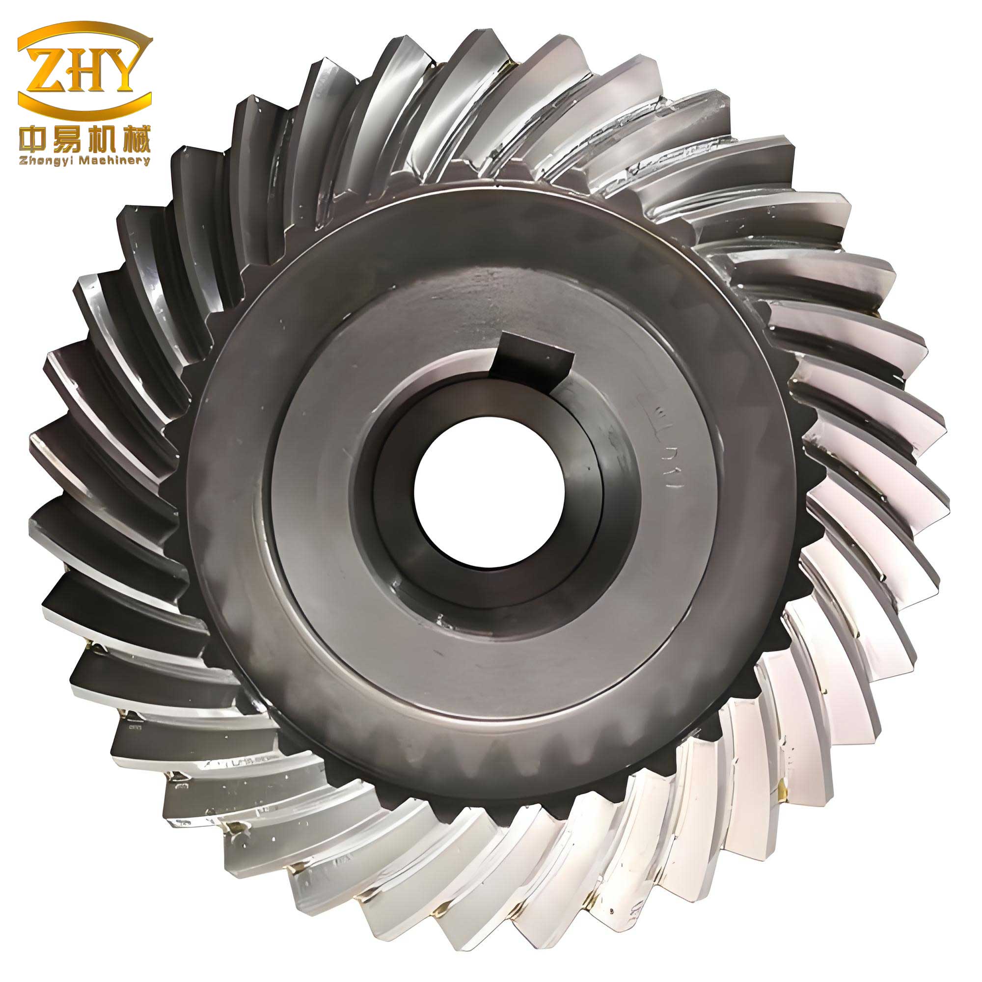
As seen in the image, spiral gears have curved teeth that engage gradually, reducing impact and noise. The spiral angle is evident from the curvature along the face width. In design, we must ensure that the spiral angles on mating gears are compatible to avoid edge contact and ensure proper load sharing.
Next, I will provide a detailed example from the provided content, translated and expanded. The original examples involved specific numbers. Let’s take one: speed ratio $i = 1.5$, center distance $a = 100$ mm, shaft intersection angle $\Sigma = 90^\circ$, and spiral gears with same hand. We need to find the spiral angles. Using the graphical method:
- Assume tentative tooth numbers: $N_1 = 24$, $N_2 = 36$ (since $i = 1.5$).
- For equivalent spur gears, assume a normal module, say $m_n = 4$ mm. Then, initial pitch diameters: $d_1 = 24 \times 4 / \cos \beta_1$ and $d_2 = 36 \times 4 / \cos \beta_2$. But $\beta$ unknown, so we guess $\beta_1 = \beta_2 = 45^\circ$ for $\Sigma = 90^\circ$. Then $d_1 \approx 135.8$ mm, $d_2 \approx 203.6$ mm, giving $a \approx 169.7$ mm, which is larger than 100 mm. So, we need smaller diameters.
- Adjust tooth numbers: try $N_1 = 16$, $N_2 = 24$. Then with $\beta_1 = \beta_2 = 45^\circ$, $d_1 \approx 90.5$ mm, $d_2 \approx 135.8$ mm, $a \approx 113.15$ mm, still larger.
- Further adjust: $N_1 = 14$, $N_2 = 21$. Then $d_1 \approx 79.2$ mm, $d_2 \approx 118.8$ mm, $a \approx 99$ mm, close to 100 mm. Now, using the graphical method, draw circles with radii $r_1 = 39.6$ mm and $r_2 = 59.4$ mm (half of diameters) centered on lines at $90^\circ$. The distance between centers should be $a = 100$ mm. Place centers accordingly. Draw tangents to the circles such that they intersect on the center line. Measure the angles from the geometry to find $\beta_1$ and $\beta_2$. Suppose from the drawing, we find $\beta_1 \approx 40^\circ$ and $\beta_2 \approx 50^\circ$. Check: $\Sigma = 40^\circ + 50^\circ = 90^\circ$, good. Then recalculate diameters with these angles: $d_1 = 14 \times 4 / \cos 40^\circ \approx 73.1$ mm, $d_2 = 21 \times 4 / \cos 50^\circ \approx 130.7$ mm, $a = 101.9$ mm, close enough. Fine-tune by adjusting $m_n$ to $3.9$ mm: then $d_1 \approx 71.3$ mm, $d_2 \approx 127.4$ mm, $a = 99.35$ mm. Thus, the spiral gears are designed.
This example shows how the graphical method guides the selection of tooth numbers and spiral angles. It is iterative but effective.
To formalize the process, I often use the following equations for spiral gears design verification. After graphical determination, compute the actual center distance using:
$$a_{\text{calc}} = \frac{m_n}{2} \left( \frac{N_1}{\cos \beta_1} + \frac{N_2}{\cos \beta_2} \right)$$
Compare with desired $a$. If not equal, adjust $m_n$ or $\beta$. The normal module $m_n$ is usually chosen from standard series, so adjusting $\beta$ is more common. The relationship between $\beta_1$ and $\beta_2$ for same hand gears is $\beta_2 = \Sigma – \beta_1$. Substitute into the center distance formula to solve for $\beta_1$:
$$a = \frac{m_n}{2} \left( \frac{N_1}{\cos \beta_1} + \frac{N_2}{\cos (\Sigma – \beta_1)} \right)$$
This equation can be solved numerically. For opposite hand, $\beta_2 = \beta_1 – \Sigma$ or $\beta_2 = \Sigma + \beta_1$, depending on which is larger. So, the formula becomes:
$$a = \frac{m_n}{2} \left( \frac{N_1}{\cos \beta_1} + \frac{N_2}{\cos (\beta_1 – \Sigma)} \right) \quad \text{(for $\beta_1 > \Sigma$)}$$
These equations highlight the complexity, justifying graphical methods.
Now, let’s create a table summarizing the steps of the graphical method for spiral gears:
| Step | Action | Purpose |
|---|---|---|
| 1 | Select tentative tooth numbers $N_1$ and $N_2$ based on speed ratio. | To establish initial gear sizes. |
| 2 | Choose a normal module $m_n$ (often from standards). | To scale the gear dimensions. |
| 3 | Draw shaft axes lines intersecting at angle $\Sigma$. | To represent the spatial arrangement of spiral gears. |
| 4 | Mark gear centers along one axis at distance $a$ apart. | To set the center distance. |
| 5 | Draw circles with radii based on equivalent pitch diameters. | To visualize the pitch circles of equivalent spur gears. |
| 6 | Draw tangents to the circles such that they intersect on the center line. | To satisfy the meshing condition for spiral gears. |
| 7 | Measure distances from centers to tangent points to compute spiral angles. | To determine $\beta_1$ and $\beta_2$ geometrically. |
| 8 | If tangents do not align, adjust tooth numbers or circle sizes and repeat. | To iteratively achieve proper design. |
| 9 | Verify with formulas for center distance and spiral angles. | To ensure accuracy of the spiral gears design. |
Beyond the graphical method, we must consider manufacturing constraints for spiral gears. The spiral angle affects the cutting tool setup and the gear generation process. For example, in Gleason or Klingelnberg methods, the spiral angle is a key parameter in machine settings. Therefore, after graphical design, we need to check feasibility in production. Typically, spiral angles are rounded to standard values like 0°, 15°, 30°, 45°, etc., to simplify tooling.
Another aspect is the contact ratio of spiral gears. The contact ratio increases with spiral angle, improving smoothness. The formula for transverse contact ratio is:
$$m_t = \frac{\sqrt{r_{a1}^2 – r_{b1}^2} + \sqrt{r_{a2}^2 – r_{b2}^2} – a \sin \alpha_t}{p_t}$$
where $r_a$ is addendum radius, $r_b$ is base radius, $\alpha_t$ is transverse pressure angle, and $p_t$ is transverse pitch. For spiral gears, the normal pressure angle is often used, and conversions are needed. The graphical method indirectly affects these by determining the pitch diameters and spiral angles.
In practice, when designing spiral gears, I also consider the axial thrust generated. The axial force $F_a$ is given by $F_a = F_t \tan \beta$, where $F_t$ is the tangential force. Therefore, higher spiral angles require stronger thrust bearings. This trade-off influences the selection of spiral angles. In the graphical method, if we aim for smaller spiral angles to reduce thrust, we might choose larger tooth numbers, which increases pitch diameters and may affect center distance. Thus, the design is a balancing act.
To illustrate with more examples, let’s consider a case from the content: speed ratio $i = 2$, center distance $a = 120$ mm, shaft intersection angle $\Sigma = 60^\circ$, spiral gears with opposite hand. Using graphical method:
- Assume $N_1 = 20$, $N_2 = 40$. For opposite hand, $\Sigma = |\beta_1 – \beta_2| = 60^\circ$. Guess $\beta_1 = 40^\circ$, then $\beta_2 = 100^\circ$ or $\beta_2 = -20^\circ$ (not practical). So, try $\beta_1 = 50^\circ$, then $\beta_2 = 10^\circ$ (since $50^\circ – 10^\circ = 40^\circ$, not 60°). Adjust: $\beta_1 = 70^\circ$, $\beta_2 = 10^\circ$ gives difference 60°. But spiral angles are typically between 0° and 45°, so this might be unrealistic. Hence, we need to adjust tooth numbers.
- Try $N_1 = 15$, $N_2 = 30$. Then, using graphical method, draw circles with radii proportional to tooth numbers. After several trials, we might find $\beta_1 \approx 35^\circ$ and $\beta_2 \approx 25^\circ$ for same hand? No, for opposite hand, $\Sigma = 60^\circ = |35^\circ – 25^\circ| = 10^\circ$, not matching. So, reverse: $\beta_1 = 45^\circ$, $\beta_2 = 15^\circ$ gives 30° difference. To get 60°, we need $\beta_1 = 75^\circ$ and $\beta_2 = 15^\circ$, but 75° is too high. Therefore, for opposite hand with $\Sigma = 60^\circ$, it’s challenging to have reasonable spiral angles. This might indicate that same hand design is preferred for this shaft angle. The graphical method helps reveal such issues early.
This underscores the importance of the graphical method in exploring feasible regions for spiral gears design.
For educational purposes, I often use software to simulate the graphical method. However, hand-drawing remains valuable for understanding. In the digital age, we can use CAD tools to perform similar constructions accurately. The principle is the same: create circles, tangents, and adjust parameters until conditions are met. The key formulas are embedded in the geometry.
Now, let’s discuss the correction factors mentioned in the content. In spiral gears design, after graphical determination, we might apply corrections to the spiral angles to account for approximations. For example, if the computed center distance is slightly off, we can adjust the spiral angles using the derivative of the center distance equation. Suppose we have initial angles $\beta_1^0$ and $\beta_2^0$, and the center distance error $\Delta a = a_{\text{calc}} – a_{\text{desired}}$. Then, small changes $\Delta \beta_1$ and $\Delta \beta_2$ can be found from:
$$\Delta a \approx \frac{\partial a}{\partial \beta_1} \Delta \beta_1 + \frac{\partial a}{\partial \beta_2} \Delta \beta_2$$
where
$$\frac{\partial a}{\partial \beta_1} = \frac{m_n N_1 \sin \beta_1}{2 \cos^2 \beta_1}, \quad \frac{\partial a}{\partial \beta_2} = \frac{m_n N_2 \sin \beta_2}{2 \cos^2 \beta_2}$$
For same hand gears, $\Delta \beta_2 = -\Delta \beta_1$ (since $\beta_1 + \beta_2 = \Sigma$ constant). So,
$$\Delta a \approx \left( \frac{m_n N_1 \sin \beta_1}{2 \cos^2 \beta_1} – \frac{m_n N_2 \sin \beta_2}{2 \cos^2 \beta_2} \right) \Delta \beta_1$$
Solve for $\Delta \beta_1$ to correct the angles. This analytical correction complements the graphical method for spiral gears.
In summary, the design of spiral gears is a multifaceted process that blends art and science. The graphical method provides a visual and intuitive way to determine spiral angles and tooth numbers, especially when dealing with indeterminate equations. By using equivalent spur gear representations and iterative adjustments, we can achieve designs that meet center distance, shaft angle, and speed ratio requirements. Throughout this article, I have emphasized the role of spiral angles in the performance of spiral gears and shown how graphical techniques can be applied with formulas and tables. Whether you are a novice or an experienced engineer, mastering these methods will enhance your ability to design efficient and reliable spiral gears for various mechanical systems.
As a final note, always remember that spiral gears are just one type of gear for intersecting shafts. Others include straight bevel gears and hypoid gears. However, spiral gears offer a unique combination of strength and smoothness, making them ideal for many applications. I hope this comprehensive guide has deepened your understanding of spiral gears design. Keep exploring and applying these principles to create innovative gear solutions.