
In this paper, I delve into the intricate mechanics of Klingelnberg hyperbolic gear systems, focusing on the derivation and implications of gear ratio correction factors and limit pressure angles. Hyperbolic gears, specifically the Klingelnberg cyclo-palloid system, offer unique advantages in power transmission due to their extended epicycloidal tooth profile and constant tooth height. These gears are widely used in industrial applications where high precision and efficiency are paramount. The analysis presented here is based on fundamental meshing principles, and I aim to provide a comprehensive understanding that can aid in the design and optimization of hyperbolic gear transmissions.
The Klingelnberg hyperbolic gear system is characterized by its use of a planar generating gear during cutting, which eliminates tooth profile errors associated with crown gear methods. This leads to simplified adjustment calculations, ease of contact pattern control, and reduced tooling requirements, making it ideal for small-batch production. Throughout this discussion, I will frequently refer to hyperbolic gear properties to emphasize their significance in mechanical engineering. The core of this study revolves around two key parameters: the gear ratio correction factor and the limit pressure angle, both of which critically influence the performance and durability of hyperbolic gear transmissions.
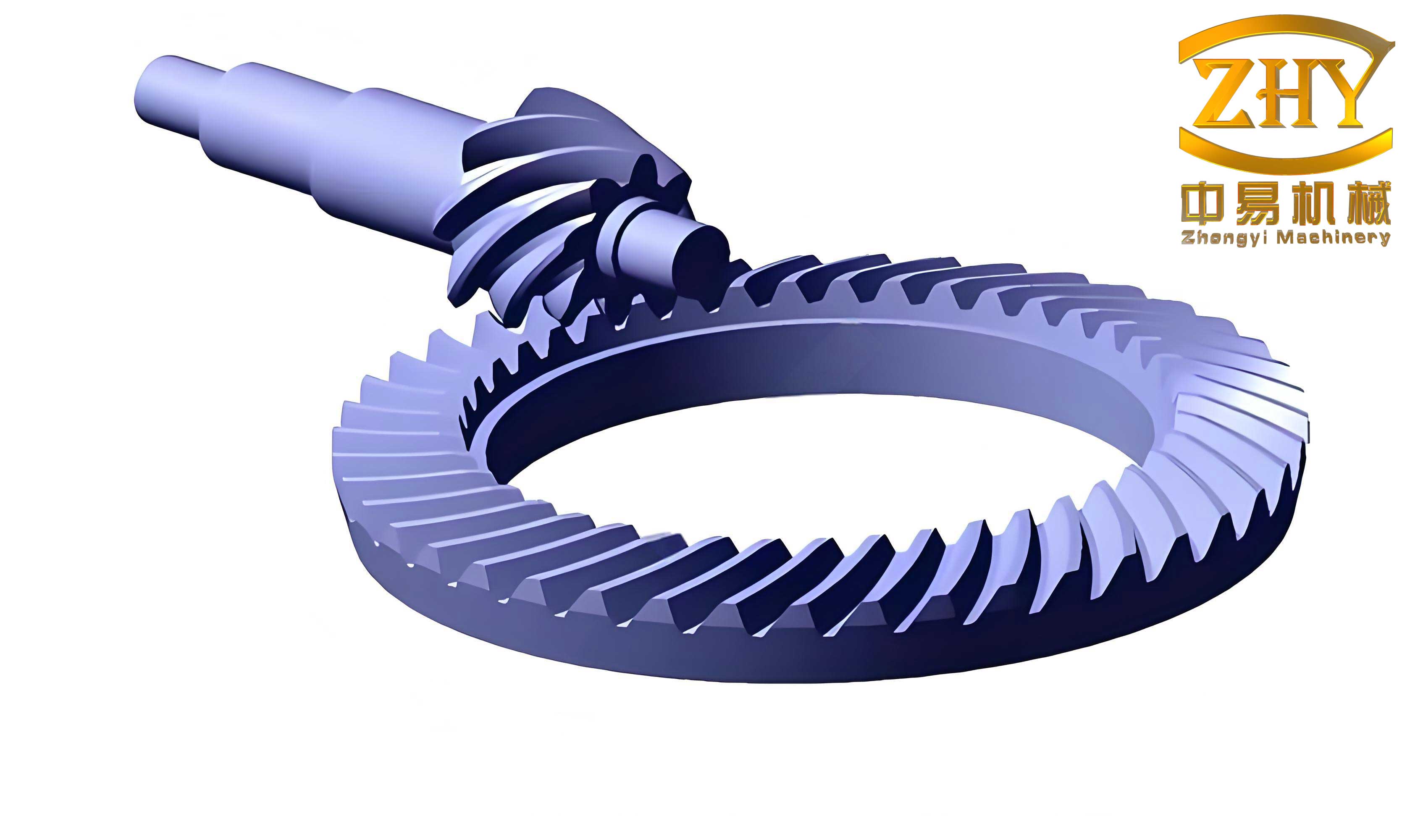
To begin, I consider the geometry of a hyperbolic gear pair. Let us define the coordinate system and parameters as follows. For a pair of Klingelnberg hyperbolic gears, the pinion and gear have their own pitch cones with apex points O1 and O2, respectively. The meshing point P is located at the midpoint of the tooth width. The axes of the pinion and gear intersect at an angle θ, and the offset angle ξ represents the projection angle between O1P and O2P in the pitch plane. The spiral angles at point P for the pinion and gear are β1 and β2, respectively. The pitch cone angles are δ1 and δ2, and the mean pitch diameters at P are d1 and d2. This setup is crucial for analyzing the kinematics of hyperbolic gear transmission.
Based on the meshing theory, the relative velocity at point P must be perpendicular to the common normal of the tooth surfaces. I derive the gear ratio correction factor by equating the relative velocity components. The angular velocities of the pinion and gear are ω1 and ω2, respectively. The velocity vectors at P are given by:
$$ \mathbf{V}_1 = \omega_1 \times \mathbf{l}_1, \quad \mathbf{V}_2 = \omega_2 \times \mathbf{l}_2 $$
where \(\mathbf{l}_1\) and \(\mathbf{l}_2\) are position vectors from the axis intersection points to P. After algebraic manipulation, the condition for meshing leads to:
$$ \omega_1 d_1 \sin \delta_1 \cos \beta_1 – \omega_2 d_2 \sin \delta_2 \cos \beta_2 = 0 $$
Simplifying, I obtain the gear ratio expression:
$$ \frac{\omega_2}{\omega_1} = \frac{d_1 \cos \beta_1}{d_2 \cos \beta_2} = F \frac{d_1}{d_2} $$
where \(F\) is the gear ratio correction factor defined as:
$$ F = \frac{\cos \beta_1}{\cos \beta_2} $$
This result highlights a key feature of hyperbolic gear systems: the gear ratio depends not only on the mean pitch diameters but also on the spiral angles of both gears. In contrast, conventional bevel gears have a fixed ratio once the diameters are set. This flexibility allows designers to adjust the transmission ratio by varying spiral angles without compromising gear strength, which is particularly beneficial in applications requiring customized speed reductions. The hyperbolic gear design thus offers enhanced versatility.
To further explore the implications, I present a table summarizing the effects of spiral angles on the gear ratio correction factor for hyperbolic gear pairs. This table illustrates how changes in β1 and β2 influence F, thereby affecting the overall transmission ratio.
| Pinion Spiral Angle β1 (degrees) | Gear Spiral Angle β2 (degrees) | Correction Factor F | Impact on Gear Ratio |
|---|---|---|---|
| 30 | 20 | 1.064 | Increases ratio |
| 35 | 25 | 1.066 | Moderate increase |
| 40 | 30 | 1.072 | Significant increase |
| 25 | 35 | 0.940 | Decreases ratio |
| 20 | 40 | 0.839 | Substantial decrease |
As shown, the correction factor F deviates from unity when spiral angles differ, allowing for ratio tuning. This is a distinct advantage of hyperbolic gear systems over traditional designs. Moreover, the inequality of spiral angles between pinion and gear in hyperbolic gear transmissions improves meshing performance by reducing sliding friction and enhancing load distribution. In practical applications, such as automotive differentials or industrial machinery, this can lead to longer service life and higher efficiency. The hyperbolic gear’s ability to accommodate varying ratios through spiral angle adjustments makes it a preferred choice in advanced transmission systems.
Next, I investigate the limit pressure angle in hyperbolic gear transmissions. The limit pressure angle, denoted α_ny, is the pressure angle at the meshing boundary point (second-kind limit point) where the tooth surfaces may cease to have full contact. Ensuring that the actual pressure angle remains within safe limits is crucial to prevent partial tooth contact, which can cause noise, vibration, and premature failure. Using meshing principles, I derive the limit pressure angle by analyzing the relative angular velocity and velocity vectors at point P.
The relative angular velocity vector ω12 is given by:
$$ \boldsymbol{\omega}_{12} = \boldsymbol{\omega}_2 – \boldsymbol{\omega}_1 = \omega_2 \left[ \left( \cos \delta_2 \cos \beta_2 + \frac{z_2}{z_1} \cos \delta_1 \cos \beta_1 \right) \mathbf{i} + \left( \cos \delta_2 \sin \beta_2 + \frac{z_2}{z_1} \cos \delta_1 \sin \beta_1 \right) \mathbf{j} – \left( \sin \delta_2 – \frac{z_2}{z_1} \sin \delta_1 \right) \mathbf{k} \right] $$
The velocity vectors are as previously defined. By computing the cross products ω12 × V2 and V12 × ω2, and summing them to form vector q, I impose the condition for the limit point: q · n_ny = 0, where n_ny is the unit normal vector at the limit point with components cos α_ny j + sin α_ny k. After simplification, I arrive at the formula for the limit pressure angle:
$$ \tan \alpha_{ny} = \frac{d_2 \sin \beta_2 \sin \delta_1 – d_1 \sin \delta_2 \sin \beta_1}{\cos \xi (d_2 \cos \delta_1 + d_1 \cos \delta_2)} = \frac{1}{\cos \xi} \frac{d_1 \sin \beta_2 \sin \delta_1 – d_2 \sin \delta_2 \sin \beta_1}{d_2 \cos \delta_1 + d_1 \cos \delta_2} $$
This equation reveals that the limit pressure angle depends solely on geometric parameters: the offset angle ξ, spiral angles β1 and β2, pitch cone angles δ1 and δ2, and mean pitch diameters d1 and d2. Importantly, it is independent of tooth profile parameters such as pressure angle or module. This underscores the fundamental nature of limit pressure angle in hyperbolic gear design. Typically, α_ny is negative, indicating that to avoid boundary points, the actual pressure angle must be carefully selected during design.
To illustrate the relationships, I present a table showing how variations in key parameters affect the limit pressure angle for a hyperbolic gear pair. This table helps designers understand the sensitivity of α_ny to different factors.
| Parameter | Value Range | Effect on Limit Pressure Angle α_ny | Design Implication for Hyperbolic Gear |
|---|---|---|---|
| Offset Angle ξ | 10° to 30° | Increases magnitude as ξ decreases | Larger offset reduces risk of boundary contact |
| Pinion Spiral Angle β1 | 20° to 40° | Decreases α_ny with increasing β1 | Higher β1 may necessitate pressure angle adjustment |
| Gear Spiral Angle β2 | 20° to 40° | Increases α_ny with increasing β2 | Balancing β1 and β2 is crucial for hyperbolic gear |
| Pitch Cone Angle δ1 | 15° to 30° | Moderate influence on α_ny | Affects load distribution in hyperbolic gear |
| Mean Diameter Ratio d1/d2 | 0.3 to 0.7 | Significant impact on α_ny magnitude | Key factor in hyperbolic gear strength design |
From this analysis, it is clear that the limit pressure angle is a critical consideration in hyperbolic gear transmission design. If not properly accounted for, it can lead to localized tooth contact, reducing efficiency and increasing wear. In practice, designers must optimize parameters like offset angle and spiral angles to ensure full tooth engagement and equal strength between mating gears. The hyperbolic gear’s unique geometry allows for such optimizations, but it requires careful calculation to avoid pitfalls.
Expanding on the meshing dynamics, I now discuss the broader implications of these findings for hyperbolic gear systems. The gear ratio correction factor F enables flexible transmission design, which is especially useful in applications where space constraints or specific speed requirements exist. For instance, in wind turbine gearboxes or aerospace mechanisms, hyperbolic gears can be tailored to achieve desired ratios without altering overall dimensions. Additionally, the limit pressure angle analysis provides a safeguard against inadequate meshing, ensuring reliability in high-load environments. The hyperbolic gear’s ability to handle offset axes further enhances its applicability in compact drive systems.
To deepen the understanding, I derive additional formulas related to hyperbolic gear performance. The contact ratio, for example, can be expressed in terms of spiral angles and pressure angles. For a hyperbolic gear pair, the transverse contact ratio m_t is approximated by:
$$ m_t = \frac{\sqrt{d_1^2 + d_2^2 – 2 d_1 d_2 \cos \xi}}{p \cos \alpha} $$
where p is the circular pitch and α is the operating pressure angle. This formula highlights how the offset angle ξ influences contact duration, which is vital for smooth operation of hyperbolic gear transmissions. Similarly, the bending stress σ_b in hyperbolic gear teeth can be estimated using the Lewis formula modified for spiral angles:
$$ \sigma_b = \frac{F_t}{b m_n Y} \cdot \frac{1}{\cos \beta_m} $$
where F_t is the tangential force, b is face width, m_n is normal module, Y is the form factor, and β_m is the mean spiral angle. These equations underscore the importance of spiral angles in hyperbolic gear design, affecting both kinematics and strength.
In terms of manufacturing, the Klingelnberg hyperbolic gear system offers advantages due to its cyclo-palloid tooth generation. The cutting process uses a planar gear, which simplifies tooling and reduces errors. I can summarize the key manufacturing parameters in a table to illustrate the relationships.
| Manufacturing Parameter | Typical Value for Hyperbolic Gear | Effect on Tooth Quality |
|---|---|---|
| Cutter Blade Angle | 20° pressure angle | Determines tooth profile accuracy |
| Machine Setting Angle | Adjustable based on δ and β | Influences contact pattern on hyperbolic gear |
| Tool Diameter | Standardized per module | Affects tooth thickness and strength |
| Spiral Angle Adjustment | ±5° tolerance | Critical for achieving desired F in hyperbolic gear |
These parameters must be tightly controlled to ensure the hyperbolic gear meets performance specifications. The flexibility of the Klingelnberg system allows for fine-tuning during production, which is beneficial for custom applications. Moreover, the use of hyperbolic gears in high-precision fields like robotics or medical equipment demands rigorous attention to these details.
Now, let’s consider numerical examples to solidify the concepts. Suppose a hyperbolic gear pair has the following parameters: d1 = 50 mm, d2 = 100 mm, β1 = 35°, β2 = 25°, δ1 = 20°, δ2 = 40°, and ξ = 15°. Using the derived formulas, I calculate the gear ratio correction factor and limit pressure angle. First, the correction factor F is:
$$ F = \frac{\cos 35^\circ}{\cos 25^\circ} = \frac{0.8192}{0.9063} = 0.904 $$
Thus, the gear ratio is:
$$ \frac{\omega_2}{\omega_1} = 0.904 \times \frac{50}{100} = 0.452 $$
This indicates a speed reduction, and the ratio is influenced by the spiral angles. Next, the limit pressure angle α_ny is computed as:
$$ \tan \alpha_{ny} = \frac{1}{\cos 15^\circ} \cdot \frac{50 \sin 25^\circ \sin 20^\circ – 100 \sin 40^\circ \sin 35^\circ}{100 \cos 20^\circ + 50 \cos 40^\circ} $$
Plugging in values: sin 25° = 0.4226, sin 20° = 0.3420, sin 40° = 0.6428, sin 35° = 0.5736, cos 20° = 0.9397, cos 40° = 0.7660, cos 15° = 0.9659. Then numerator: 50 × 0.4226 × 0.3420 = 7.22, 100 × 0.6428 × 0.5736 = 36.86, so difference = -29.64. Denominator: 100 × 0.9397 + 50 × 0.7660 = 93.97 + 38.30 = 132.27. Thus, tan α_ny = (1/0.9659) × (-29.64/132.27) = 1.035 × (-0.224) = -0.232, so α_ny = -13.1°. This negative value confirms the need to design the actual pressure angle appropriately to avoid boundary points in this hyperbolic gear pair.
These calculations demonstrate the practical application of the derived formulas. Designers can use such analyses to optimize hyperbolic gear transmissions for specific needs. Furthermore, I explore the impact of temperature and lubrication on hyperbolic gear performance, though these factors are beyond the scope of the core equations. However, it’s worth noting that the meshing characteristics of hyperbolic gears make them less sensitive to misalignment compared to straight bevel gears, enhancing their robustness in variable conditions.
In conclusion, the Klingelnberg hyperbolic gear system offers significant advantages through its adjustable gear ratio and controllable limit pressure angle. The gear ratio correction factor F, dependent on spiral angles, provides flexibility in transmission design, allowing for ratio changes without altering gear diameters. The limit pressure angle, determined by offset angle, spiral angles, pitch cone angles, and diameters, serves as a critical check to ensure full tooth contact and equal strength. These insights are essential for advancing hyperbolic gear technology in modern engineering applications. Future work could involve finite element analysis to validate stress distributions or experimental studies on noise reduction in hyperbolic gear transmissions. Ultimately, the continued development of hyperbolic gear systems will rely on a deep understanding of these fundamental principles, driving innovation in power transmission solutions.
To summarize key equations for hyperbolic gear design, I list them below for quick reference:
- Gear Ratio: $$ \frac{\omega_2}{\omega_1} = \frac{d_1 \cos \beta_1}{d_2 \cos \beta_2} = F \frac{d_1}{d_2} $$
- Correction Factor: $$ F = \frac{\cos \beta_1}{\cos \beta_2} $$
- Limit Pressure Angle: $$ \tan \alpha_{ny} = \frac{d_2 \sin \beta_2 \sin \delta_1 – d_1 \sin \delta_2 \sin \beta_1}{\cos \xi (d_2 \cos \delta_1 + d_1 \cos \delta_2)} $$
- Transverse Contact Ratio: $$ m_t = \frac{\sqrt{d_1^2 + d_2^2 – 2 d_1 d_2 \cos \xi}}{p \cos \alpha} $$
- Bending Stress (simplified): $$ \sigma_b = \frac{F_t}{b m_n Y} \cdot \frac{1}{\cos \beta_m} $$
These formulas encapsulate the core mechanics of hyperbolic gear transmissions. By integrating them into design software, engineers can efficiently develop optimized hyperbolic gear systems for diverse industries. The ongoing research in this field promises to further enhance the efficiency and reliability of hyperbolic gears, solidifying their role in advanced mechanical systems.
Finally, I emphasize that the study of hyperbolic gear transmissions is not merely academic but has practical ramifications. From automotive differentials to industrial mixers, the ability to tailor gear ratios and ensure robust meshing through limit pressure angle control makes hyperbolic gears a versatile choice. As technology evolves, the demand for compact, high-performance transmissions will only increase, and hyperbolic gear systems are well-positioned to meet these challenges. Through continued analysis and innovation, we can unlock even greater potentials for hyperbolic gear applications, driving progress in engineering and manufacturing worldwide.