
Herringbone gears are widely employed in high-speed and heavy-duty applications such as marine propulsion and aerospace transmissions, because they combine the high load-carrying capacity of helical gears with the elimination of net axial thrust. In practice, the two helical halves of a herringbone gear are manufactured separately on the same blank, and unavoidable manufacturing errors lead to a lack of symmetry between the left-hand and right-hand tooth flanks. This symmetry deviation is known to cause uneven load distribution, increased contact stress, additional axial vibration, and reduced service life, especially in high-speed aviation gear drives. However, standardized definitions, evaluation methods, and inspection procedures for the symmetry deviation of herringbone gears are still lacking in many countries. In this paper, I systematically investigate the characterization, measurement, and data processing methods for the symmetry deviation of herringbone gears, and I evaluate the influence of different symmetry deviation components on the meshing behavior. The main contributions of this work are: (1) proposing a multi-component characterization of symmetry deviation based on the symmetry mid-plane; (2) developing a coordinate-measuring-machine (CMM) based measurement strategy and a dedicated data processing program; (3) experimentally verifying the proposed method on three aviation herringbone gears; and (4) establishing finite-element contact models to compare the influence of circumferential, radial, and angular deviation components. The results indicate that the proposed definitions and measurement procedures can effectively quantify the symmetry deviation of herringbone gears and provide useful guidance for design and quality control.
The rest of this paper is organized as follows. In Section 1, I review the background and existing research on gear metrology and herringbone gear errors. In Section 2, I formulate the symmetry deviation problem and derive the characterization model. In Section 3, I present the measurement principle, the selection of feature lines, and the program design. In Section 4, I describe the measurement experiments, data processing, and error compensation. In Section 5, I analyze the influence of symmetry deviation components on the contact behavior of herringbone gears through finite element simulations. Finally, Section 6 summarizes the conclusions and future work.
1. Background and Literature Review
Gear measurement technology has evolved from mechanical comparative methods to modern coordinate metrology. Single-error measurements, such as profile, helix, and pitch deviations, are widely used in quality control. Composite error measurements and gear integrated error measurements provide a more global view of gear quality. CNC gear measuring centers and coordinate measuring machines (CMMs) allow three-dimensional evaluation of complex tooth surfaces. Non-contact optical methods are also emerging, though contact probing remains the most reliable for high-precision gear metrology.
Many researchers have studied the influence of gear errors on the dynamic behavior and load distribution. Manufacturing errors, such as pitch deviation, profile deviation, helix deviation, and eccentricity, affect the transmission error, mesh stiffness, and vibration response of gear systems. For herringbone gears, the axial symmetry between the two helical halves is a critical factor. Some studies introduced concepts such as alignment deviation, symmetry deviation, and centering error to describe the relative position of the left-hand and right-hand tooth flanks. However, these concepts often focus on a single scalar value, such as the distance between the extrapolated helix lines at the symmetry plane, while ignoring angular misalignments in the profile and helix directions. Therefore, a more complete characterization is needed.
In the field of herringbone gear measurement, several methods have been proposed. One approach measures the median line of the tooth space and uses the intersection of the tooth flank with the symmetry mid-plane. Another method defines the symmetry deviation as the distance between the midpoints of two corresponding points on the left and right helical flanks. Some researchers have also suggested using the tooth contact line to evaluate symmetry. However, most of these approaches are either too complex, require high precision repeated probing, or do not fully capture the three-dimensional nature of the deviation. There is also a lack of standard measurement procedures. Therefore, this paper aims to fill this gap by providing a systematic method.
2. Characterization of Symmetry Deviation for Herringbone Gears
2.1 Problem Transformation
Consider an ideal herringbone gear. If one half is mirrored with respect to the symmetry mid-plane, it should coincide exactly with the other half. In reality, manufacturing errors cause the actual tooth flanks of the two halves to differ. Therefore, the symmetry deviation of herringbone gears can be transformed into a comparison between the mirrored left-hand flank and the actual right-hand flank (or vice versa). This comparison is analogous to the comparison between an actual tooth flank and a theoretical tooth flank in conventional gear metrology. According to gear error theory, a three-dimensional deviation between two flanks can be decomposed into a distance deviation and two angular deviations. Thus, the following formulation is established.
2.2 Basic Gear Error Definitions
For a single helical gear, the tooth flank is generated by sweeping an involute curve along a helix. The standard involute equation in polar coordinates is
$$ r_k = \frac{r_b}{\cos \alpha_k}, \qquad \theta_k = \operatorname{inv}\alpha_k = \tan\alpha_k – \alpha_k, $$
where \(r_b\) is the base-circle radius, \(\alpha_k\) is the pressure angle at point \(k\), and \(\theta_k\) is the roll angle. In Cartesian coordinates, the involute is expressed as
$$ \begin{cases}
x_k = r_b(\cos \varphi_k + \varphi_k \sin \varphi_k), \\
y_k = r_b(\sin \varphi_k – \varphi_k \cos \varphi_k),
\end{cases} $$
where \(\varphi_k = \theta_k + \alpha_k\). For a helical gear, the tooth flank is obtained by rotating the involute along the helix. If the helix angle is \(\beta\), and the rotation angle around the gear axis is \(\gamma\), the flank coordinates become
$$ \begin{cases}
x_p = r_b(\cos \varphi_k + \varphi_k \sin \varphi_k)\cos\gamma – r_b(\sin \varphi_k – \varphi_k \cos\varphi_k)\sin\gamma, \\
y_p = r_b(\cos \varphi_k + \varphi_k \sin \varphi_k)\sin\gamma + r_b(\sin \varphi_k – \varphi_k \cos\varphi_k)\cos\gamma, \\
z_p = r_b \, \gamma \, \cot\beta.
\end{cases} $$
The profile deviation and helix deviation of a gear are defined according to ISO standards. The total profile deviation \(F_\alpha\), profile form deviation \(f_{f\alpha}\), and profile slope deviation \(f_{H\alpha}\) are the common indices. Similarly, the total helix deviation \(F_\beta\), helix form deviation \(f_{f\beta}\), and helix slope deviation \(f_{H\beta}\) are used for the helix direction. These definitions provide the basis for the comparison of the two halves of herringbone gears.
2.3 Decomposition of Symmetry Deviation
When the mirrored left-hand flank is compared with the right-hand flank, the differences can be classified into four fundamental components:
- Circumferential distance deviation \(L_s\) – the angular phase difference between the two flanks at the same radius and height, converted to an arc length on the reference circle.
- Radial distance deviation \(L_R\) – the difference in the radial positions of the two flanks, often caused by a difference in the effective base-circle radius.
- Helix angle deviation \(L_\alpha\) – the angular misalignment of the flank in the helix direction, expressed as an equivalent length over the measured face width.
- Profile angle deviation \(L_\beta\) – the angular misalignment of the flank in the involute profile direction, expressed as an equivalent length over the measured profile range.
The physical meanings of these four components are illustrated conceptually in the following table.
| Component | Symbol | Physical meaning | Unit |
|---|---|---|---|
| Circumferential distance deviation | \(L_s\) | Phase difference converted to arc length | μm |
| Radial distance deviation | \(L_R\) | Difference in radial distance from gear axis | μm |
| Helix angle deviation | \(L_\alpha\) | Helix-direction angular misalignment | μm |
| Profile angle deviation | \(L_\beta\) | Profile-direction angular misalignment | μm |
2.4 Calculation Formulas
Let the two mean helix lines of the left and right flanks, after mirroring, intersect the symmetry mid-plane at points \(A_1(x_1,y_1,z_1)\) and \(A_2(x_2,y_2,z_2)\). These points have polar coordinates \((R_1,\theta_1)\) and \((R_2,\theta_2)\):
$$ R_1 = \sqrt{x_1^2 + y_1^2}, \qquad \theta_1 = \arctan(y_1/x_1), $$
$$ R_2 = \sqrt{x_2^2 + y_2^2}, \qquad \theta_2 = \arctan(y_2/x_2). $$
The radial distance deviation is
$$ L_R = R_1 – R_2. $$
The phase difference is
$$ \Delta\varphi = \theta_1 – \theta_2, $$
and the circumferential distance deviation is evaluated at the reference radius \(r_b\):
$$ L_s = r_b \, \Delta\varphi. $$
Let the mean helix angles of the two flanks be \(\alpha_1\) and \(\alpha_2\). The helix angle deviation is
$$ L_\alpha = \frac{\alpha_1 – \alpha_2}{\sin(\Delta Z)}, $$
where \(\Delta Z\) is the face width over which the helix is measured. For the profile direction, suppose the mean profile lines of the two flanks are shifted so that their starting points coincide. The angle between them is \(\Delta\beta\), and the profile angle deviation is
$$ L_\beta = \max(r_{k1}, r_{k2}) \cdot (\theta_{k1} – \theta_{k2}), $$
where \(r_{k1}\) and \(r_{k2}\) are the radii of the evaluated profile endpoints. In the experiments, all four components are computed from the measured helix and profile data.
3. Measurement Method and Program Design
3.1 Selection of Feature Lines
For measuring the symmetry deviation of herringbone gears, I compared three possible CMM point-extraction methods: feature-point measurement, feature-line measurement, and full-flank measurement. Feature-point measurement is simple but requires very high positioning accuracy and cannot capture angular deviations. Full-flank measurement provides rich information but is time-consuming and may be unnecessary for symmetry evaluation. Feature-line measurement, which extracts the helix line at the reference circle and the profile line at the face-width middle, offers a good balance between efficiency and information content. Therefore, I adopted the feature-line method.
The extraction scheme is as follows. For the helix-line measurement, the probe scans along the intersection of the tooth flank with the reference cylinder. The measurement points are spaced with equal increments along the gear axis. For the profile-line measurement, the probe scans along the intersection of the tooth flank with the mid-plane of the face width. Three equidistant strategies are possible: equal angle increments, equal radius increments, or equal involute length increments. I chose equal angle increments because it is straightforward to implement on a CMM and facilitates later calculations.
3.2 Reference System and Symmetry Mid-Plane
The symmetry mid-plane is a virtual plane that does not physically exist on the gear. Therefore, its position must be established from manufacturing datum features. For a gear with an integral shaft, two cylindrical journal surfaces and two shoulder faces are used as datum features. The procedure is as follows:
- Mount the herringbone gear on the CMM table using a suitable fixture.
- Probe several points on one cylindrical journal to define the gear axis (Z-axis).
- Probe several points on one shoulder face to define the XY plane.
- Measure the two shoulder faces (or the two end faces of the gear blank) and compute the mid-plane offset along the Z-axis.
- Translate the XY plane to the symmetry mid-plane.
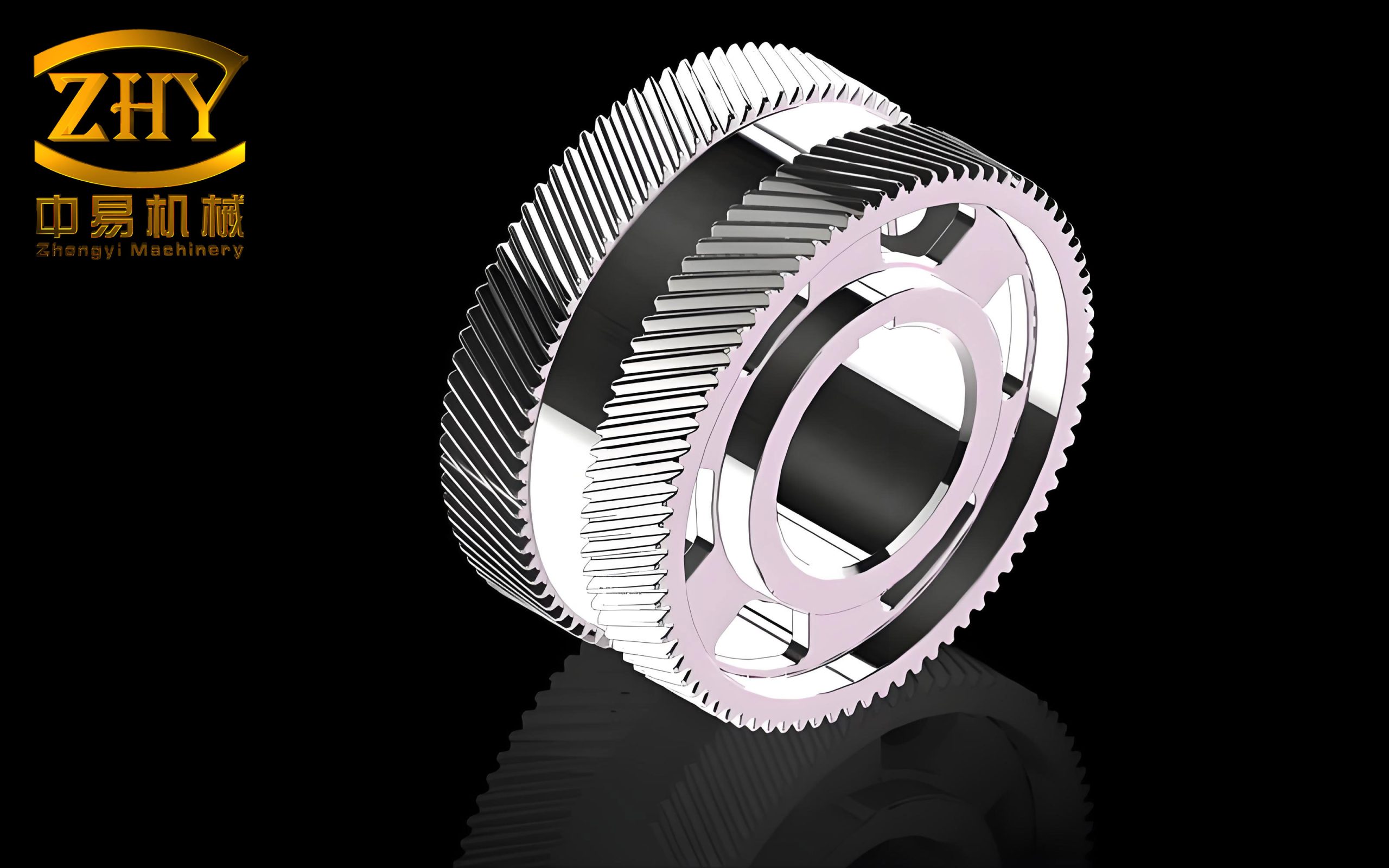
The following figure shows a typical herringbone gear used in this study. The symmetry mid-plane is indicated by the dashed plane. This figure is inserted here to illustrate the physical geometry.
3.3 Data Extraction Program
The data extraction program is based on the Quindos software environment of the CMM. A script was designed to control the probe movements and record the coordinates of the measured points. The core steps of the extraction program are:
- Calibrate the probe using a reference sphere.
- Establish the coordinate system from the datum features.
- Define the gear parameters (module, number of teeth, pressure angle, helix angle, hand of helix).
- Select the tooth flank to be measured by manually probing one point on the target flank and one point on the adjacent flank.
- Automatically scan the helix line and the profile line with the specified point density.
- Export the measured point coordinates to an Excel file for further processing.
The program allows measuring both the left-hand and right-hand flanks of the herringbone gears. The extracted data contain the Cartesian coordinates \( (x,y,z) \) of each scanned point.
3.4 Data Processing Program
The data processing program was written in MATLAB. It performs the following tasks:
- Read the measured point coordinates from the Excel file.
- Fit the mean helix line using a helical curve model.
- Fit the mean profile line using an involute curve model.
- Extrapolate the helix lines to the symmetry mid-plane and compute \(L_R\), \(L_s\), and \(L_\alpha\).
- Align the profile lines to a common starting point and compute \(L_\beta\).
- Calculate the conventional helix deviations and profile deviations for verification.
The helix line fitting was performed using the nonlinear least-squares method. The model equation is
$$ x = r\cos\theta, \qquad y = r\sin\theta, \qquad z = b\theta, $$
where \(r\) is the reference radius and \(b\) is the helix parameter. The profile line fitting uses the involute equation in Cartesian form, with the base-circle radius and the roll angle as parameters. The MATLAB script also computes the distances from each measured point to the fitted curve, which are useful for evaluating form deviations.
4. Measurement Experiments and Data Analysis
4.1 Test Gear Parameters
Three groups of aviation herringbone gears were measured in this study. The basic parameters of the test gear are listed in the table below.
| Parameter | Symbol | Value |
|---|---|---|
| Number of teeth | \(z\) | 27 |
| Normal module | \(m_n\) | 3.8788 mm |
| Normal pressure angle | \(\alpha_n\) | 22.5° |
| Helix angle | \(\beta\) | 30° |
| Tip circle diameter | \(d_a\) | 130.62 mm |
| Root circle diameter | \(d_f\) | 108.51 mm |
| Face width (per half) | \(b\) | 47 mm |
4.2 Equipment and Calibration
The measurements were performed on a Hexagon Global 575 coordinate measuring machine. The main technical specifications are listed in the table below.
| Item | Value |
|---|---|
| X-axis travel | 800 mm |
| Y-axis travel | 1000 mm |
| Z-axis travel | 600 mm |
| Maximum permissible error | \(3.0 + L/300\) μm |
| Resolution | 0.078 μm |
| Temperature | 20 ± 2 °C |
| Humidity | 45%–75% |
Before the measurement, the CMM was calibrated using grade-2 gauge blocks with nominal lengths of 400 mm, 250 mm, 200 mm, 150 mm, and 30 mm. The calibration was performed in three principal axes and four spatial diagonal directions. All calibration results were within the permissible error limits. A ruby ball stylus with a diameter of 1 mm was selected because of the small tooth space of the gear.
4.3 Helix Line Measurement Results
For one group of herringbone gears, the measured helix-line points of the left-hand and right-hand flanks were imported into MATLAB. The fitted mean helix lines are shown in relation to the symmetry mid-plane. Due to manufacturing errors, the two helix lines do not intersect the symmetry mid-plane at the same point. The deviation appears in both the circumferential and radial directions, which confirms the need for multi-component characterization.
The measured points were compared with the fitted mean helix line. The distances from the measured points to the fitted helix line are shown below. For the left-hand flank, the average distance was 6.8 μm and the maximum distance was 16.8 μm. For the right-hand flank, the average distance was 4.0 μm and the maximum distance was 20.5 μm. These values indicate the form quality of the helix lines.
Using the calculation formulas from Section 2, the following symmetry deviation components were obtained for the third group:
- Circumferential distance deviation \(L_s = 17.8\) μm
- Radial distance deviation \(L_R = 11.7\) μm
- Helix angle deviation \(L_\alpha = 7.2\) μm
- Profile angle deviation \(L_\beta = 8.4\) μm
The conventional helix deviations were also computed. For the left-hand flank: total helix deviation \(F_\beta = 23.2\) μm, helix slope deviation \(f_{H\beta} = 2.9\) μm, helix form deviation \(f_{f\beta} = 21.9\) μm. For the right-hand flank: \(F_\beta = 21.2\) μm, \(f_{H\beta} = 4.0\) μm, \(f_{f\beta} = 20.0\) μm.
4.4 Profile Line Measurement Results
The profile line measurement points were processed in a similar manner. The measured points were compared with the theoretical involute flank. In the profile evaluation range, fifty measured points were selected. The distances from these points to the theoretical profile were plotted. The left-hand flank had a profile deviation of 10.2 μm, and the right-hand flank had a profile deviation of 10.4 μm.
The profile deviations were also calculated according to ISO definitions. For the left-hand flank: total profile deviation \(F_\alpha = 10.8\) μm, profile slope deviation \(f_{H\alpha} = 6.8\) μm, profile form deviation \(f_{f\alpha} = 10.9\) μm. For the right-hand flank: \(F_\alpha = 13.4\) μm, \(f_{H\alpha} = 8.1\) μm, \(f_{f\alpha} = 9.5\) μm.
4.5 Summary of Symmetry Deviation Results
Three groups of herringbone gears were measured. The resulting symmetry deviation components are summarized in the following table.
| Group | \(L_s\) (μm) | \(L_R\) (μm) | \(L_\alpha\) (μm) | \(L_\beta\) (μm) |
|---|---|---|---|---|
| Group 1 | 15.3 | 10.2 | 5.3 | 6.3 |
| Group 2 | 13.6 | 8.5 | 6.5 | 5.9 |
| Group 3 | 17.8 | 11.7 | 7.2 | 8.4 |
According to the design drawing, the allowable centering error for the tested herringbone gears was 20 μm. The maximum measured circumferential deviation among the three groups was 17.8 μm, which indicates that the gears met the design requirement.
To verify the measurement accuracy, the helix deviations computed from the measured points were compared with the values reported by the gear measurement module of the CMM software. The comparison is shown in the table below.
| Error item | Computed by MATLAB (μm) | Quindos module (μm) |
|---|---|---|
| Helix total deviation \(F_\beta\) | 23.2 | 20.1 |
| Helix slope deviation \(f_{H\beta}\) | 2.9 | 2.5 |
| Helix form deviation \(f_{f\beta}\) | 21.9 | 21.2 |
The differences between the two sets of results are relatively small, which confirms the correctness of the proposed measurement and data processing method.
4.6 Error Source Analysis
Measurement errors in CMM-based gear inspection arise from several sources. The first is the stylus radius. Since a spherical stylus is used, the recorded coordinates correspond to the center of the sphere, not the actual contact point. The compensation formula for the probe radius in the involute direction is
$$ x_0 = x_1 – r_c \cos\alpha_a \cos\theta_a, $$
$$ y_0 = y_1 + r_c \cos\alpha_a \sin\theta_a, $$
where \(r_c\) is the stylus radius, \(\alpha_a\) is the pressure angle, and \(\theta_a\) is the roll angle. In the experiments, the compensation did not significantly change the symmetry deviation results, because the probe radius mainly shifts the measured points along the flank normal without altering the relative geometry between the two flanks.
The second error source is the CMM positioning error. The actual measured point may deviate from the intended theoretical point. Since the actual point lies on the real tooth flank, it must satisfy the flank equation. I used the gear flank equation to optimize the measured points. The optimized points were closer to the theoretical points, and the average distance decreased from 2.84 μm to 1.83 μm. The compensation also improved the stability of the data. After error compensation, the symmetry deviation components were re-calculated, as shown in the table below.
| Group | Condition | \(L_s\) (μm) | \(L_R\) (μm) | \(L_\alpha\) (μm) | \(L_\beta\) (μm) |
|---|---|---|---|---|---|
| 1 | Original | 15.3 | 10.2 | 5.3 | 6.3 |
| 1 | Compensated | 11.5 | 8.3 | 5.1 | 5.8 |
| 2 | Original | 13.6 | 8.5 | 6.5 | 5.9 |
| 2 | Compensated | 10.7 | 8.0 | 6.3 | 5.6 |
| 3 | Original | 17.8 | 11.7 | 7.2 | 8.4 |
| 3 | Compensated | 15.3 | 9.4 | 6.9 | 8.1 |
The circumferential and radial deviations were reduced by about 1–2 μm after compensation, while the angular deviations changed only slightly.
5. Influence of Symmetry Deviation on Meshing Characteristics
5.1 Modified Tooth Flank Equation
To study the influence of the symmetry deviation of herringbone gears, I extended the standard tooth flank equation by incorporating the four deviation components. The circumferential distance deviation \(L_s\) introduces an additional rotation matrix \(\mathbf{P}\) around the gear axis:
$$ \mathbf{P} =
\begin{bmatrix}
\cos\gamma_i & -\sin\gamma_i & 0 \\
\sin\gamma_i & \cos\gamma_i & 0 \\
0 & 0 & 1
\end{bmatrix}, $$
where \(\gamma_i = L_s / r_i\) and \(r_i\) is the polar radius of the flank point. The radial distance deviation \(L_R\) changes the effective base-circle radius:
$$ r_b’ = r_b + L_R. $$
The helix angle deviation \(L_\alpha\) changes the helix angle to
$$ \beta’ = \arctan\left(\frac{B \tan\beta + L_\alpha}{B}\right), $$
where \(B\) is the face width. The profile angle deviation \(L_\beta\) changes the involute starting angle by
$$ \Delta\alpha = \arctan\left(\frac{L_\beta}{L}\right), $$
where \(L\) is the profile evaluation length. Combining these effects, the modified tooth flank coordinates of herringbone gears can be written as
$$ \begin{cases}
x = r_b'(\cos\varphi_k + \varphi_k\sin\varphi_k)\cos(\gamma + \gamma_i) – r_b'(\sin\varphi_k – \varphi_k\cos\varphi_k)\sin(\gamma + \gamma_i), \\
y = r_b'(\cos\varphi_k + \varphi_k\sin\varphi_k)\sin(\gamma + \gamma_i) + r_b'(\sin\varphi_k – \varphi_k\cos\varphi_k)\cos(\gamma + \gamma_i), \\
z = r_b'(\gamma + \gamma_i)\cot\beta’.
\end{cases} $$
5.2 Finite Element Contact Analysis
Static contact analyses of herringbone gears with and without symmetry deviation were performed using Abaqus. The gear pair parameters are listed below.
| Parameter | Pinion | Wheel |
|---|---|---|
| Number of teeth | 41 | 44 |
| Normal module (mm) | 3.5 | 3.5 |
| Normal pressure angle (°) | 22.5 | 22.5 |
| Helix angle (°) | 30 | 30 |
| Face width (mm) | 30 | 30 |
| Gap width (mm) | 20 | 20 |
The model was meshed with about 300,000 elements, with local refinement at the contact regions. The material was 45 steel with elastic modulus \(E = 210\) GPa, Poisson’s ratio \(\nu = 0.3\), and density \(\rho = 7800\) kg/m\(^3\). A torque of 2 kN·m was applied. For the standard herringbone gear, the contact stress distribution was symmetric about the mid-plane. The maximum contact stress was 16621 N/m² (in the normalized simulation).
Then, four separate models were created by introducing each symmetry deviation component with two magnitudes: the measured value and the measured value increased by 50%. The values used in the simulations are listed below.
| Component | Measured value (μm) | Increased value (μm) |
|---|---|---|
| \(L_s\) | 17.8 | 26.7 |
| \(L_R\) | 11.7 | 17.6 |
| \(L_\alpha\) | 7.2 | 10.8 |
| \(L_\beta\) | 8.4 | 12.6 |
For each simulation, the stress distribution on the tooth flank was extracted. The results show that any symmetry deviation component causes the load to concentrate on one half of the herringbone gear, while the other half becomes less loaded. This leads to uneven load distribution and increased maximum contact stress. The time-varying contact stress curves were also plotted. The maximum stress values for each case are summarized in the following tables.
| Case | Maximum stress (N/m²) | Increase relative to standard (%) |
|---|---|---|
| Standard herringbone gears | 16621 | – |
| \(L_s = 17.8\) μm | 16883 | 1.58 |
| \(L_s = 26.7\) μm | 17284 | 3.99 |
| \(L_R = 11.7\) μm | 17564 | 5.67 |
| \(L_R = 17.6\) μm | 17972 | 8.12 |
| \(L_\alpha = 7.2\) μm | 17640 | 6.13 |
| \(L_\alpha = 10.8\) μm | 17808 | 7.14 |
| \(L_\beta = 8.4\) μm | 18986 | 14.2 |
| \(L_\beta = 12.6\) μm | 20697 | 24.5 |
Among the four symmetry deviation components of herringbone gears, the profile angle deviation \(L_\beta\) has the most significant effect on the maximum contact stress. Even a relatively small \(L_\beta\) of 8.4 μm increases the maximum stress by 14.2%. When \(L_\beta\) is increased to 12.6 μm, the maximum stress rises by 24.5%. Therefore, in the design and manufacturing of herringbone gears, the control of the profile angle deviation is particularly important.
6. Conclusion and Future Work
In this paper, I have presented a systematic investigation of the characterization and measurement of symmetry deviation for herringbone gears. The main conclusions are as follows:
- The symmetry deviation of herringbone gears can be transformed into a comparison between the mirrored left-hand flank and the right-hand flank. Based on gear error theory, the symmetry deviation is represented by four components: circumferential distance deviation \(L_s\), radial distance deviation \(L_R\), helix angle deviation \(L_\alpha\), and profile angle deviation \(L_\beta\). Calculation formulas were derived for each component.
- A feature-line measurement method was selected for CMM-based data extraction. The helix line at the reference cylinder and the profile line at the face-width middle were scanned. A complete measurement program was designed using the Quindos environment, and a MATLAB data processing program was developed to compute the symmetry deviation components and conventional gear deviations.
- Measurement experiments were performed on three groups of aviation herringbone gears. The computed helix deviations were compared with the values obtained by the gear measurement module, and the results were in good agreement, verifying the correctness of the proposed method. Error analysis showed that stylus-radius compensation has little influence on the symmetry deviation, while positioning-error compensation can reduce the circumferential and radial deviations by about 1–2 μm.
- Finite element contact analyses revealed that all four symmetry deviation components cause load concentration on one half of the herringbone gear and increase the maximum contact stress. Among them, the profile angle deviation \(L_\beta\) has the greatest influence on the contact stress distribution. Therefore, the profile angle deviation should be strictly controlled during the manufacturing of herringbone gears.
For future work, the following topics are suggested:
- Optimization of the measurement method to enable faster point-based symmetry deviation evaluation for production environments.
- Development of a complete error evaluation standard for the symmetry deviation of herringbone gears, similar to existing gear accuracy standards.
- Full-flank scanning of herringbone gears to study symmetry deviation in the context of gear integrated error.
- Dynamic analysis of herringbone gears with symmetry deviation to investigate the influence of each component on vibration and noise, and to establish more comprehensive design guidelines.
The research presented in this paper provides a theoretical basis and practical measurement tool for the quality control of herringbone gears. The proposed method contributes to the accurate characterization of symmetry deviation and helps improve the reliability and performance of herringbone gear transmissions.