
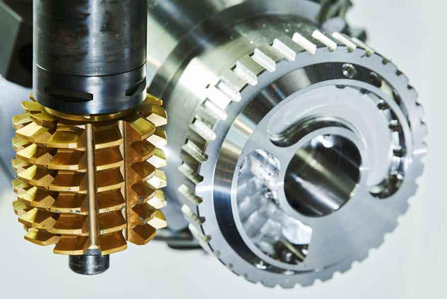
In my work on precision manufacturing, I treat gear hobbing as one of the most important generating processes for producing small-module, high-accuracy gears. Dry gear hobbing is especially attractive because it removes cutting fluid, reduces environmental burden, and supports high-speed continuous production. However, dry gear hobbing also creates a difficult thermal environment. Because high-pressure air replaces liquid cooling, the heat generated by cutting, friction, and motor losses cannot be removed efficiently. The resulting temperature gradients deform the bed, columns, hob head, worktable, and spindle system. These deformations change the relative position between the hob and the workpiece, especially along the x-axis, and therefore change the cutting depth. The final result is a gear hobbing thermal error that directly affects tooth thickness, profile accuracy, and consistency.
I classify the main error sources of a dry gear hobbing machine into four groups. Thermal error is usually the largest dynamic component. It cannot be removed by a fixed geometric correction because it develops with time, load, and cutting sequence. In my experiments, the thermal deformation grew from nearly zero to a stable level after approximately forty continuously cut gears. This behavior makes real-time detection and compensation essential for gear hobbing accuracy.
| Error source | Main cause | Nature | Typical role in gear hobbing | Possible treatment |
|---|---|---|---|---|
| Geometric error | Assembly, guideway alignment, spindle axis error | Quasi-static | Initial tooth thickness and lead deviation | Calibration and parameter correction |
| Thermal error | Cutting heat, motor heat, friction heat, poor air cooling | Dynamic and time-varying | Dominant effect on x-axis hob-workpiece distance | Real-time detection and compensation |
| Force-induced error | Cutting force, clamping force, gravity | Dynamic | Elastic deflection and vibration | Stiffness improvement and adaptive control |
| Other errors | Servo dynamics, tool wear, interpolation, chatter | Mixed | Local profile and surface errors | Condition monitoring and process optimization |
For a dry gear hobbing machine, the heat conduction process can be represented by a transient temperature field. I use the following form to describe the internal energy balance of a machine component:
$$\rho c_p \frac{\partial T}{\partial t} = \nabla \cdot \left(k \nabla T\right) + q_{gen}$$
where \(\rho\) is density, \(c_p\) is specific heat capacity, \(T\) is temperature, \(k\) is thermal conductivity, and \(q_{gen}\) is the internal heat generation rate. The boundary condition includes convection with the surrounding air:
$$-k \frac{\partial T}{\partial n} = h\left(T – T_{\infty}\right)$$
where \(h\) is the convective heat transfer coefficient and \(T_{\infty}\) is the ambient temperature. For dry gear hobbing, \(h\) is much smaller than in wet cutting, so the accumulated heat remains longer inside the structure. The thermal deformation of a machine component of length \(L\) can be approximated as:
$$\Delta L = \alpha L \Delta T$$
where \(\alpha\) is the coefficient of thermal expansion and \(\Delta T\) is the temperature rise. In a complex dry gear hobbing machine, many components deform simultaneously, so the total x-axis thermal error is a superposition of several deformation sources:
$$\Delta x_{th}(t) = \sum_{i=1}^{n} \alpha_i L_i \Delta T_i(t) + \delta_{contact}(t) + \delta_{joint}(t)$$
The term \(\delta_{contact}(t)\) represents contact interface effects, and \(\delta_{joint}(t)\) represents joint clearance effects. For gear hobbing, the x-axis error is the most important because it changes the center distance between the hob and the gear blank. If the x-axis error is \(\varepsilon_x\), the deviation along the base circle tangent on the gear end face is:
$$PP’ = \varepsilon_x \sin \alpha$$
where \(\alpha\) is the normal pressure angle. For a standard pressure angle of \(20^\circ\), a small x-axis thermal error produces a measurable tooth profile deviation. This is why I focus on real-time detection and compensation of the x-axis thermal error in dry gear hobbing.
I analyzed the structural layout of a high-speed dry gear hobbing machine. The main heat sources are the main spindle motor, the hob spindle motor, the direct-drive torque motor of the worktable, the cutting zone, and the guideway friction. Heat is transferred through the bed, columns, hob head, and worktable. Because the machine is not geometrically symmetrical, the temperature distribution is non-uniform. The bed may elongate, the columns may bend or tilt, and the hob head may shift. These effects combine to change the hob-workpiece distance during gear hobbing. The thermal error develops slowly at first, then accelerates, and finally reaches a plateau when the heat generation and heat dissipation become balanced.
To measure this thermal deformation directly, I designed a direct detection method based on a compact laser displacement sensor. The sensor is mounted below the hob head through a fixed plate. A pneumatic cylinder, an ejector pin, a guide rail, and a fixture box form the motion and positioning unit. After each gear hobbing cycle, the CNC system sends a detection command. The pneumatic cylinder pushes the sensor along the guide rail to a specified measuring position. The laser beam then measures the distance between the hob head reference and a selected point on the workpiece fixture. This distance change is used to represent the thermal deformation of the dry gear hobbing machine.
| Component | Function in direct detection | Key requirement |
|---|---|---|
| Laser displacement sensor | Measures hob head to fixture distance | Micrometer resolution and fast response |
| Fixed plate | Connects sensor to hob head | High stiffness and thermal stability |
| Pneumatic cylinder | Moves sensor to measurement position | Repeatable stroke and stable pressure |
| Guide rail | Guides sensor motion | Low friction and high straightness |
| Fixture box | Protects sensor and provides reference | Rigid support and chip protection |
| Data interface | Transmits distance data to PC | Reliable serial communication |
The direct detection value can be written as:
$$d_m(t) = d_0 + \Delta x_{th}(t) + \epsilon_m(t)$$
where \(d_m(t)\) is the measured distance, \(d_0\) is the initial reference distance, \(\Delta x_{th}(t)\) is the thermal deformation along the x-axis, and \(\epsilon_m(t)\) is measurement noise. The thermal deformation is therefore estimated as:
$$\Delta x_{th}(t) = d_m(t) – d_0 – \epsilon_m(t)$$
I also set a compensation threshold \(T_c\). When the absolute thermal deformation exceeds this threshold, the compensation system generates a correction. The detection logic is:
$$\text{Compensation action} =
\begin{cases}
1, & |\Delta x_{th}(t)| \ge T_c \\
0, & |\Delta x_{th}(t)| < T_c
\end{cases}$$
For the software side of the direct detection method, I developed a Windows application in C#. The program includes network communication with the CNC system, serial port configuration, data acquisition, data judgment, and display. The main workflow is as follows: initialize the serial port, open the connection, read the CNC macro variable that acts as a software switch, send a measurement request to the laser sensor, receive the distance value, calculate the minimum distance in the measurement window, compare it with the baseline, and decide whether to write a compensation value. The software switch is important because the sensor should not measure during gear hobbing. It should only measure after the hob has moved away from the cutting zone.
| Step | Action | Output or decision |
|---|---|---|
| 1 | Initialize serial port and network connection | Ready state |
| 2 | Read CNC macro variable as software switch | Start or wait |
| 3 | Send measurement request to laser sensor | Distance data stream |
| 4 | Receive and parse distance data | Distance sequence |
| 5 | Compute minimum distance and deformation | Thermal error estimate |
| 6 | Compare with threshold | Compensation decision |
| 7 | Write compensation macro variable | CNC correction value |
Although direct detection is accurate, it can disturb the production cycle because the sensor must move into a special measuring position after each gear. It also adds hardware cost and mechanical complexity. For this reason, I also developed an indirect method based on machine characterization signals. In this method, I collect spindle current signals and thermal key-point temperature signals during gear hobbing. Then I build a mapping model from these signals to the thermal deformation state. Once the model is trained, I can estimate the thermal error in real time without stopping the gear hobbing process for a dedicated measurement stroke.
The signal acquisition system contains Hall current sensors, PT100 thermal resistance sensors, a data acquisition card, a junction box, and a PC. Two Hall current sensors monitor the spindle current. Six PT100 sensors monitor selected thermal key points. The thermal key points are chosen according to previous thermal analysis of the dry gear hobbing machine. The current signals are analog values, so the data acquisition system performs analog-to-digital conversion and sends the digital data to the PC. The temperature sensors and the laser displacement sensor communicate with the PC through serial communication.
| Signal | Sensor | Quantity | Purpose |
|---|---|---|---|
| Spindle current | Hall current sensor | 2 channels | Cutting load and process state |
| Thermal key-point temperature | PT100 | 6 channels | Thermal state of machine structure |
| Thermal deformation | Laser displacement sensor | 1 channel | Direct label for model training |
| Process trigger | Eddy current sensor | 1 channel | Mark the start of gear hobbing |
The spindle current is a three-phase signal. I use the root mean square value to represent the effective current. For one phase, the RMS value is:
$$I_{rms,a}(t) = \sqrt{\frac{1}{N}\sum_{k=1}^{N} i_a^2(k)}$$
For the three-phase system, I use:
$$I_{rms}(t) = \sqrt{\frac{i_a^2(t) + i_b^2(t) + i_c^2(t)}{3}}$$
where \(i_a\), \(i_b\), and \(i_c\) are the instantaneous currents of the three phases. During a single gear hobbing cycle, the current rises as the hob enters the gear blank, reaches a maximum when the contact length is large, and then decreases as the hob exits. The current waveform therefore contains information about cutting load, tool-workpiece interaction, and thermal state. However, the current signal alone is not enough. Temperature signals provide a slower but more direct view of the thermal state. I combine current and temperature data to improve the robustness of thermal error monitoring in dry gear hobbing.
Before feature extraction, I clean the raw data. Missing values are removed or interpolated. Outliers caused by chip interference or sensor noise are filtered. Then I normalize each signal to a common scale. The min-max normalization is:
$$x’ = \frac{x – x_{min}}{x_{max} – x_{min}}$$
This step prevents large amplitude variables from dominating the model. It also improves the convergence of neural network training. After cleaning and normalization, I extract features from the current signal in the time domain, frequency domain, and time-frequency domain. I also include temperature features. The combined feature set is designed to capture both fast dynamic changes and slow thermal trends in gear hobbing.
Time-domain features are simple and fast to compute. They reflect amplitude, dispersion, and shape. I use the following time-domain parameters for the spindle current signal.
| Feature | Expression | Meaning |
|---|---|---|
| Mean | \(\bar{x}=\frac{1}{N}\sum_{i=1}^{N}x_i\) | Average level |
| RMS | \(x_{rms}=\sqrt{\frac{1}{N}\sum_{i=1}^{N}x_i^2}\) | Effective energy |
| Variance | \(\sigma^2=\frac{1}{N}\sum_{i=1}^{N}(x_i-\bar{x})^2\) | Dispersion |
| Standard deviation | \(\sigma=\sqrt{\sigma^2}\) | Amplitude fluctuation |
| Skewness | \(S=\frac{1}{N}\sum_{i=1}^{N}\left(\frac{x_i-\bar{x}}{\sigma}\right)^3\) | Asymmetry |
| Kurtosis | \(K=\frac{1}{N}\sum_{i=1}^{N}\left(\frac{x_i-\bar{x}}{\sigma}\right)^4\) | Peakedness |
| Peak | \(x_p=\max |x_i|\) | Maximum amplitude |
| Waveform factor | \(W=\frac{x_{rms}}{|\bar{x}|}\) | Waveform shape |
| Crest factor | \(C=\frac{x_p}{x_{rms}}\) | Peak severity |
| Impulse factor | \(I=\frac{x_p}{|\bar{x}|}\) | Impulse content |
| Clearance factor | \(CL=\frac{x_p}{\left(\frac{1}{N}\sum_{i=1}^{N}\sqrt{|x_i|}\right)^2}\) | Clearance condition |
| Kurtosis factor | \(K_f=\frac{K}{x_{rms}^4}\) | Normalized kurtosis |
Frequency-domain features reveal how the signal energy is distributed over frequency. For a continuous current signal \(x(t)\), the Fourier transform is:
$$X(f) = \int_{-\infty}^{\infty} x(t) e^{-j2\pi f t} dt$$
In practical computation, I use the discrete Fourier transform:
$$X(k) = \sum_{n=0}^{N-1} x(n) e^{-j2\pi kn/N}$$
and the fast Fourier transform to reduce computation. The frequency-domain features I use include centroid frequency, mean square frequency, and frequency variance.
| Frequency feature | Expression | Interpretation |
|---|---|---|
| Centroid frequency | \(F_c=\frac{\sum_{k=1}^{K} f_k S(k)}{\sum_{k=1}^{K} S(k)}\) | Center of spectral energy |
| Mean square frequency | \(F_{ms}=\frac{\sum_{k=1}^{K} f_k^2 S(k)}{\sum_{k=1}^{K} S(k)}\) | Energy-weighted frequency |
| Frequency variance | \(F_v=\frac{\sum_{k=1}^{K}(f_k-F_c)^2 S(k)}{\sum_{k=1}^{K} S(k)}\) | Spread of spectral energy |
Time-frequency analysis is necessary because the spindle current in gear hobbing is non-stationary. The cutting load changes continuously as the hob rotates and translates. I first apply wavelet packet denoising to the current signal. The mother wavelet is defined as:
$$\psi_{a,b}(t) = \frac{1}{\sqrt{|a|}} \psi\left(\frac{t-b}{a}\right)$$
where \(a\) is the scale factor and \(b\) is the translation factor. The continuous wavelet transform is:
$$W(a,b) = \int_{-\infty}^{\infty} x(t) \psi_{a,b}^{*}(t) dt$$
For discrete signals, I use the discrete wavelet transform and wavelet packet decomposition. Wavelet packet decomposition divides the full frequency band into multiple levels and provides a more detailed local representation than ordinary wavelet decomposition. After denoising, I apply empirical mode decomposition to obtain intrinsic mode functions. An IMF must satisfy two conditions: the number of extrema and zero crossings must be equal or differ by at most one, and the mean of the upper and lower envelopes must be zero. The current signal can be decomposed as:
$$x(t) = \sum_{i=1}^{n} c_i(t) + r_n(t)$$
where \(c_i(t)\) are IMF components and \(r_n(t)\) is the residual. For each IMF component, I compute the energy:
$$E_i = \sum_{k=1}^{N} |c_i(k)|^2$$
The energy values of the IMF components form a compact representation of the time-frequency content. I use sixteen IMF energy values as features. Together with time-domain features, frequency-domain features, and temperature features, they form a multi-domain feature set for gear hobbing thermal error monitoring.
| Domain | Feature group | Number of features |
|---|---|---|
| Time domain | Mean, RMS, variance, standard deviation, skewness, kurtosis, peak, waveform factor, crest factor, impulse factor, clearance factor, kurtosis factor | 14 |
| Frequency domain | Centroid frequency, mean square frequency, frequency variance | 3 |
| Time-frequency domain | IMF energy values after wavelet packet denoising and EMD | 16 |
| Thermal domain | Selected thermal key-point temperatures | 3 |
| Total | Combined feature vector | 36 |
With the 36-dimensional feature vector, I first built a traditional BP neural network model. A BP network is a multilayer feedforward network trained by error backpropagation. It has an input layer, one or more hidden layers, and an output layer. Neurons in the same layer are not connected, while neurons in adjacent layers are fully connected. For the \(l\)-th layer, the net input of neuron \(j\) is:
$$z_j^{(l)} = \sum_{i} w_{ji}^{(l)} a_i^{(l-1)} + b_j^{(l)}$$
The activation output is:
$$a_j^{(l)} = f\left(z_j^{(l)}\right)$$
where \(f\) is the activation function. The training error for one sample is:
$$E = \frac{1}{2}\sum_{k=1}^{m}\left(y_k – \hat{y}_k\right)^2$$
The weights are updated by gradient descent:
$$w_{ji}^{(l)} \leftarrow w_{ji}^{(l)} – \eta \frac{\partial E}{\partial w_{ji}^{(l)}}$$
where \(\eta\) is the learning rate. The backpropagation process uses the chain rule to propagate the output error backward and adjust weights and biases. Although BP networks are universal approximators, they can fall into local minima, converge slowly, and depend strongly on the quality of the feature set. In my dry gear hobbing thermal error task, the BP model provided a baseline but not the best final performance.
| Hidden layers | Neurons in hidden layer 1 | Neurons in hidden layer 2 | Neurons in hidden layer 3 | Training error |
|---|---|---|---|---|
| 1 | 8 | – | – | 0.341 |
| 1 | 12 | – | – | 0.281 |
| 1 | 16 | – | – | 0.264 |
| 2 | 8 | 4 | – | 0.322 |
| 2 | 12 | 4 | – | 0.198 |
| 2 | 16 | 4 | – | 0.263 |
| 3 | 8 | 8 | 4 | 0.289 |
| 3 | 12 | 8 | 4 | 0.201 |
| 3 | 16 | 8 | 4 | 0.224 |
According to the experimental comparison, I selected a BP network with two hidden layers. The first hidden layer had 12 neurons, and the second hidden layer had 4 neurons. The input layer had 36 neurons, and the output layer had 3 neurons representing the thermal deformation state. The maximum number of iterations was set to 100,000, the learning rate was 0.1, and the target error was 0.18. The network was trained multiple times to evaluate robustness.
| Network trial | Recognition rate for thermal deformation above threshold | Recognition rate for thermal deformation below threshold |
|---|---|---|
| 1 | 0.922 | 0.844 |
| 2 | 0.884 | 0.951 |
| 3 | 0.861 | 0.896 |
| 4 | 0.853 | 0.913 |
| 5 | 0.854 | 0.902 |
| 6 | 0.912 | 0.889 |
| 7 | 0.896 | 0.942 |
The recognition rate for the below-threshold class was generally higher because the data set contained more samples in that class. In gear hobbing thermal error control, however, the cost of a missed positive detection is much higher than the cost of a false positive. If the thermal deformation exceeds the threshold but the model fails to detect it, the gear may be cut with an uncorrected error. If the model falsely triggers compensation, the loss is usually smaller. I therefore defined a weighted evaluation cost:
$$C = 0.85 C_{1} + 0.15 C_{2}$$
where \(C_1\) is the cost of a false negative and \(C_2\) is the cost of a false positive. Using this evaluation, the average accuracy of the BP model was approximately 82.39%. This result was useful but not sufficient for a high-speed dry gear hobbing machine. The main limitations were local minima, limited feature representation, and a relatively small training sample set.
To improve the thermal error detection performance, I investigated deep learning models. I first considered a deep autoencoder built from stacked restricted Boltzmann machines. A restricted Boltzmann machine has a visible layer and a hidden layer. Connections exist only between layers, not within a layer. For visible units \(v_i\) and hidden units \(h_j\), the energy function is:
$$E(v,h) = -\sum_i a_i v_i – \sum_j b_j h_j – \sum_{i,j} v_i w_{ij} h_j$$
The joint probability is:
$$P(v,h) = \frac{1}{Z} e^{-E(v,h)}$$
where \(Z\) is the partition function. Because there are no intra-layer connections, the conditional probabilities are simple:
$$P(h_j=1 \mid v) = \sigma\left(b_j + \sum_i v_i w_{ij}\right)$$
$$P(v_i=1 \mid h) = \sigma\left(a_i + \sum_j h_j w_{ij}\right)$$
where \(\sigma(x)=1/(1+e^{-x})\) is the sigmoid function. Stacking several RBMs forms a deep autoencoder. The training process is greedy and layer-wise. After pretraining, the network is fine-tuned by backpropagation. The reconstruction loss for an autoencoder is:
$$L_{sq} = \|x – \hat{x}\|^2$$
or, for binary-like features, the cross-entropy loss is:
$$L_{ce} = -\sum_{i}\left[x_i \log \hat{x}_i + (1-x_i)\log(1-\hat{x}_i)\right]$$
I tested several hidden-layer configurations for the deep autoencoder. The input dimension was 36. The two RBM hidden layers were varied. The best configuration in my tests was 36-150-150-20, but the overall accuracy was still limited by the small sample size and the fact that the handcrafted features could not fully represent the dry gear hobbing thermal state.
| RBM1 hidden neurons | RBM2 hidden neurons | Model accuracy |
|---|---|---|
| 100 | 10 | 0.6591 |
| 150 | 10 | 0.6885 |
| 200 | 10 | 0.6742 |
| 100 | 20 | 0.6962 |
| 150 | 20 | 0.8857 |
| 200 | 20 | 0.8282 |
| 100 | 30 | 0.6874 |
| 150 | 30 | 0.8126 |
| 200 | 30 | 0.7236 |
Because the deep autoencoder did not reach the desired accuracy, I then developed a convolutional neural network model combined with a deep autoencoder classifier. The idea was to use the CNN to learn local patterns from a signal image formed by the spindle current time-domain waveform and the temperature signals. This avoids relying only on handcrafted features and allows the model to discover discriminative patterns related to gear hobbing thermal error.
The CNN model has three important properties: local connection, weight sharing, and spatial or temporal sampling. A convolutional layer replaces full connections with local receptive fields. The convolution operation for a one-dimensional signal can be written as:
$$y_j^{(l)} = f\left(\sum_{i=1}^{M} x_i^{(l-1)} * k_{ij}^{(l)} + b_j^{(l)}\right)$$
where \(x_i^{(l-1)}\) is the input feature map, \(k_{ij}^{(l)}\) is the convolution kernel, \(b_j^{(l)}\) is the bias, and \(*\) denotes convolution. The pooling operation reduces the feature dimension:
$$p_j^{(l)} = \max_{r \in R} y_j^{(l)}(r)$$
or it can use average pooling. After several convolution and pooling layers, the learned feature maps are flattened into a one-dimensional vector. This vector is then input to a deep autoencoder for classification. The deep autoencoder contains an encoder, a decoder, and hidden layers. The encoder maps input \(x\) to a latent representation \(h\):
$$h = f_{\theta}(x)$$
The decoder reconstructs the input:
$$\hat{x} = g_{\theta’}(h)$$
The training objective is to minimize the reconstruction error and the classification error. In my CNN-DAE model, the network was trained by unsupervised pretraining followed by supervised fine-tuning. The training process can be summarized as follows.
| Stage | Operation | Purpose |
|---|---|---|
| 1 | Input current and temperature signal image | Preserve raw process information |
| 2 | Convolution and pooling | Extract local and hierarchical features |
| 3 | Flatten feature maps | Convert multidimensional features to a vector |
| 4 | DAE hidden layers | Learn compact thermal error representation |
| 5 | Softmax output layer | Classify thermal deformation state |
| 6 | Backpropagation fine-tuning | Reduce classification error |
I trained the CNN-DAE model with the mixed time-domain signal image. The input combined spindle current waveforms and temperature signals. The model learned to distinguish different thermal deformation states. After multiple iterations, the average accuracy reached approximately 0.9124. This was higher than both the BP network and the DAE model. The result showed that the CNN-DAE model could capture more useful thermal information from the raw signal image than the handcrafted feature set alone, especially in the complex and non-stationary process of dry gear hobbing.
| Model | Input form | Average accuracy | Main limitation |
|---|---|---|---|
| BP neural network | 36-dimensional multi-domain feature vector | 0.8239 | Local minima and limited feature expression |
| Deep autoencoder | 36-dimensional multi-domain feature vector | 0.8857 | Small sample size and feature limitation |
| CNN-DAE | Current and temperature signal image | 0.9124 | Higher computational cost |
After selecting the CNN-DAE model as the thermal error detection model, I designed a real-time compensation system for the dry gear hobbing machine. The compensation principle is simple: the model estimates the thermal deformation along the x-axis, and the CNC system applies an equal and opposite correction to the x-axis position. The compensation value is:
$$\Delta x_{comp}(t) = -\Delta \hat{x}_{th}(t)$$
where \(\Delta \hat{x}_{th}(t)\) is the estimated thermal error from the CNN-DAE model. Because the thermal error changes slowly compared with the cutting cycle, the compensation is updated after each gear hobbing cycle or when the estimated error exceeds the threshold. This keeps the actual hob-workpiece distance close to the ideal value.
The compensation hardware includes the dry gear hobbing machine, Hall current sensors, PT100 temperature sensors, a data acquisition card, a junction box, a PC, and the FANUC CNC system. The signal acquisition system collects current and temperature data in real time. The PC processes the data, forms the signal image, feeds it into the trained CNN-DAE model, and obtains the thermal error estimate. If compensation is needed, the PC communicates with the CNC system and writes the correction value into a macro variable.
| Hardware | Role | Interface |
|---|---|---|
| Dry gear hobbing machine | Production process | Mechanical and CNC |
| Hall current sensors | Spindle current measurement | Analog to DAQ |
| PT100 sensors | Thermal key-point measurement | Serial or DAQ |
| Data acquisition card | Analog-to-digital conversion | PXI or PCI |
| Junction box | Signal connection | Wired |
| PC | Model inference and compensation decision | Ethernet and serial |
| FANUC CNC | Axis motion and macro execution | FOCAS Ethernet |
I used the FANUC FOCAS library to communicate between the PC and the CNC system. FOCAS provides functions to open a connection, read macro variables, and write macro variables. The relevant functions include:
$$ \text{cnc\_allclibhndl3}(ip, port, timeout, handle) $$
$$ \text{cnc\_rdmacro}(handle, number, length, macro) $$
$$ \text{cnc\_wrmacro}(handle, number, length, value, decimal\_offset) $$
I selected macro variable #841 as the software switch for the measurement or compensation cycle. When the hob moves to the safe position, the CNC sets #841 to 1. When the machine returns to cutting, #841 is set to 0. I selected macro variable #842 as the compensation value output. The compensation value is written as an integer with a decimal offset. For example, a value of \(-15\) with decimal offset \(3\) represents \(-0.015\) mm.
| Macro variable | Type | Use in my compensation system |
|---|---|---|
| #0 | Null | Always empty |
| #1 to #33 | Local variable | Macro-local storage |
| #100 to #199 | Common variable | Shared but cleared after power-off |
| #500 to #999 | Common variable | Shared and retained after power-off |
| #1000 and above | System variable | CNC status and control data |
| #841 | Common variable | Software switch for measurement/compensation |
| #842 | Common variable | Thermal error compensation value |
The upper-computer software was developed in C# as a Windows Forms application. It includes serial communication, Ethernet communication, data parsing, thermal error estimation, and macro variable writing. The workflow starts with initialization. The program detects available serial ports, sets the baud rate, and opens the port. It then opens a FOCAS handle to the CNC. A background thread reads macro variable #841. When the value is 1, the program starts a measurement or estimation cycle. In the direct detection mode, the program sends a request code to the laser displacement sensor, receives distance data, and computes the minimum distance. In the indirect mode, the program uses the trained CNN-DAE model to estimate the thermal error from current and temperature signals. When the absolute error exceeds the threshold, the program writes the compensation value to macro #842. Otherwise, it writes zero or no compensation.
| Software module | Function | Key implementation |
|---|---|---|
| Serial communication | Laser sensor and temperature data | SerialPort object and data receive event |
| Ethernet communication | CNC connection | FOCAS handle and macro read/write |
| Data processing | Cleaning, normalization, feature image | Min-max scaling and image construction |
| Thermal error model | CNN-DAE inference | Pre-trained weights and biases |
| Compensation decision | Threshold comparison | Absolute error and cost-sensitive logic |
| Macro writing | Write value to CNC | cnc_wrmacro with decimal offset |
To evaluate the compensation system, I cut fifty gear blanks continuously on the dry gear hobbing machine. The thermal error developed from nearly zero to a stable value. I measured the M value of the cut gears to represent tooth thickness accuracy. The M value is sensitive to the x-axis distance between the hob and the workpiece. When the machine becomes hotter, the x-axis distance increases, the cutting depth decreases, and the M value increases. When compensation is applied, the CNC moves the x-axis in the opposite direction, so the M value decreases.
| Gear number | Thermal trend | Compensation action | Observed M-value response |
|---|---|---|---|
| 1 to 10 | Initial heating, small deformation | None | M value gradually increases |
| 12 | First threshold crossing | Compensation applied | M value decreases |
| 20 | Continued heating | Compensation applied | M value decreases |
| 28 | Approaching thermal equilibrium | Compensation applied | M value decreases |
| 32 | Near-equilibrium correction | Compensation applied | M value decreases |
| 40 to 50 | Thermal equilibrium | Intermittent correction | M value remains within about 0.02 mm |
The compensation events at gears 12, 20, 28, and 32 produced clear downward jumps in the M value. Because gear hobbing also involves tool wear, blank allowance variation, and force-induced deflection, the M value still showed some fluctuation. However, the overall trend confirmed that the thermal error was being detected and corrected. After the machine reached thermal equilibrium, the M value remained within an acceptable band. This demonstrated that real-time thermal error detection and compensation improved the consistency of dry gear hobbing.
From my results, I conclude that thermal error is the dominant dynamic error in dry gear hobbing. The direct laser detection method provides accurate labels and can be used for calibration. The indirect signal-based method is more suitable for production because it does not interrupt the gear hobbing cycle. The combination of spindle current, temperature, and multi-domain features gives a practical representation of the thermal state. Traditional BP networks provide a baseline, but deep learning models, especially the CNN-DAE model, achieve higher accuracy because they can learn hierarchical features from the signal image. The compensation system based on FOCAS macro variables is simple, low-cost, and compatible with industrial CNC systems. It can write correction values during gear hobbing and reduce the effect of thermal deformation on tooth thickness.
Several directions remain for future work. First, I plan to extract more comprehensive multi-domain features and apply statistical purification methods such as principal component analysis and correlation analysis. This may reduce redundancy and improve the thermal representation capability of the feature set. Second, I plan to collect more data across more production batches so that the deep learning model can be trained on a larger and more diverse sample set. Third, I intend to integrate other error sources such as vibration, tool wear, and blank allowance variation into a unified gear hobbing error model. This would allow compensation to address not only thermal error but also the coupled effects that appear in real dry gear hobbing production. Finally, I will continue to optimize the real-time inference speed and the communication reliability of the compensation system so that it can be deployed on high-speed dry gear hobbing machines with minimal production impact.