
In the realm of mechanical engineering and design, the spiral bevel gear stands as a quintessential component characterized by its complex, spatially curved tooth surfaces. These gears are pivotal in transmitting power between intersecting axes, often at right angles, with high efficiency and smooth operation. The design and manufacturing of spiral bevel gears have traditionally been challenging due to their intricate geometry. However, with the advent of advanced computer-aided design (CAD) software like Pro/ENGINEER (Pro/E), it has become feasible to create accurate three-dimensional models that can be seamlessly integrated into virtual environments for structural analysis, assembly simulation, and computer-aided manufacturing (CAM). This article delves into my comprehensive methodology for achieving full three-dimensional parametric modeling of spiral bevel gears within the Pro/E environment. The approach leverages Pro/E’s robust surface modeling capabilities, its embedded programming language Pro/Program, and parametric relations to create a flexible design system. By inputting fundamental gear parameters such as module, number of teeth, spiral angle, pressure angle, and cutter radius, a corresponding accurate 3D solid model of the spiral bevel gear is automatically generated. This parametric framework not only streamlines the design process but also serves as a foundational digital twin for subsequent engineering applications like finite element analysis (FEA) and numerical control (NC) programming.
The core of modeling any gear lies in mathematically defining its tooth profile. For a spiral bevel gear, the theoretical tooth flank is derived from a spherical involute. This is because the gear teeth are formed on a spherical surface, making the spherical coordinate system the most natural and efficient framework for their mathematical description. In Pro/E, complex curves can be defined using equation-driven curves, where the spherical coordinates—radial distance (\( \rho \)), polar angle (\( \theta \)), and azimuthal angle (\( \phi \))—are expressed as functions of a parameter \( t \) (typically ranging from 0 to 1). The fundamental equations for the tooth profile at the gear’s outer end (or heel) are established as follows.
The radial distance \( \rho \) for the outer sphere is constant and is defined by the module \( m \) and the number of teeth \( z \). For a gear pair with pinion teeth \( z_1 \) and gear teeth \( z_2 \), the spherical radius \( R \) (which is the outer cone distance) is calculated as:
$$ R = \frac{m \cdot z_1}{2} \cdot \sqrt{1 + \left( \frac{z_2}{z_1} \right)^2 } $$
The polar angle \( \theta \) corresponds to the cone angle, which varies from the root cone angle \( \Gamma_f \) to the face cone angle \( \Gamma_a \). The most critical component is the azimuthal angle \( \phi \), which describes the spherical involute. For any point \( p \) on the involute with a cone angle \( \Gamma_p \), the angle \( \phi_p \) is given by:
$$ \phi_p = \frac{1}{\sin \Gamma_b} \cdot \arccos \left( \frac{\cos \Gamma_p}{\cos \Gamma_b} \right) – \arccos \left( \frac{\tan \Gamma_b}{\tan \Gamma_p} \right) $$
Here, \( \Gamma_b \) is the base cone angle of the spiral bevel gear. This equation is central to generating the accurate tooth flank geometry. The base cone angle is derived from the pitch cone angle \( \Gamma \) and the normal pressure angle \( \alpha_n \):
$$ \Gamma_b = \arcsin(\sin \Gamma \cdot \cos \alpha_n) $$
These formulas provide the mathematical foundation for constructing the tooth surfaces in the CAD environment.
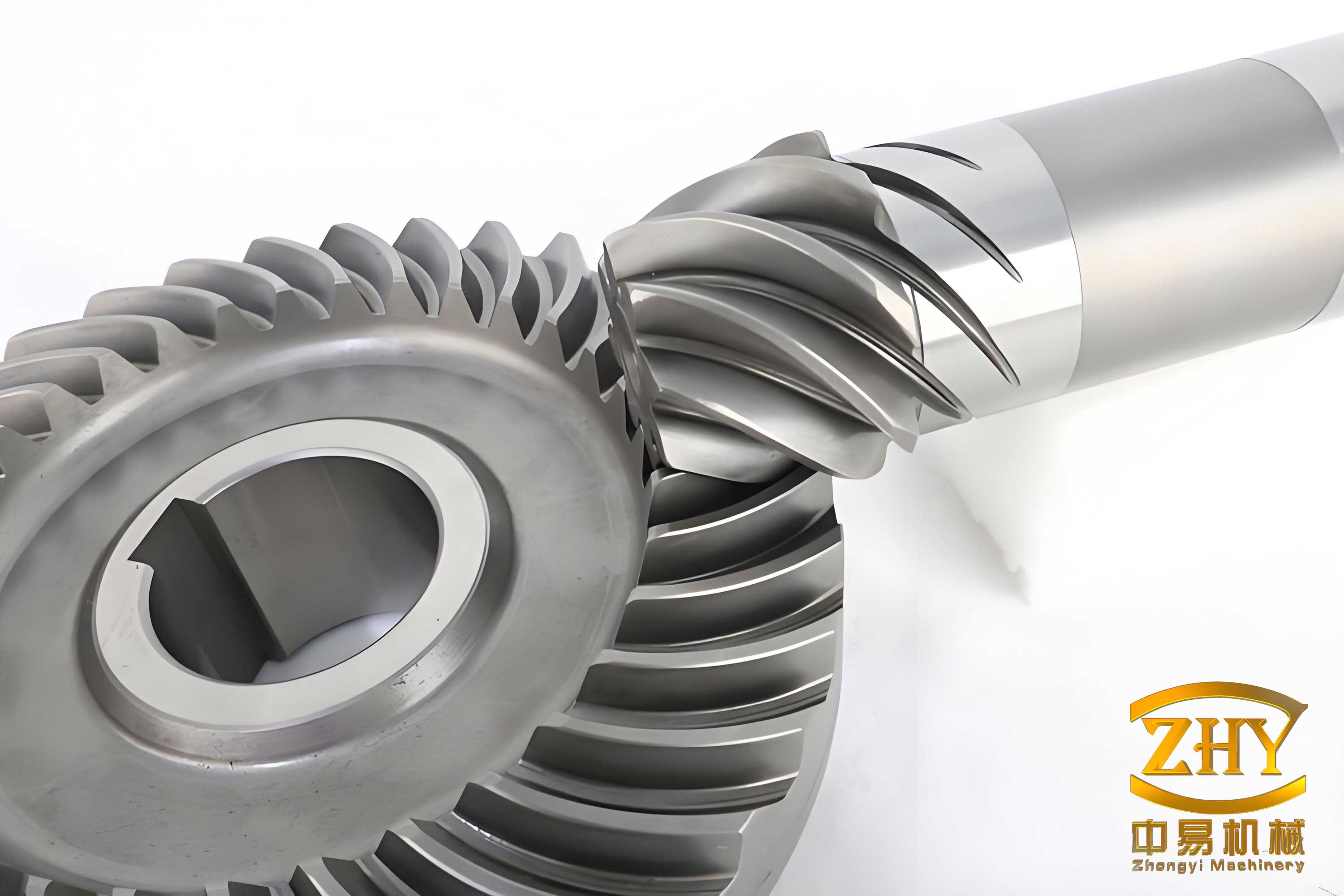
The modeling process for a single tooth of the spiral bevel gear is systematic and involves creating a network of bounding curves to define a surface patch. The first step is to create the spherical involute curves at the outer heel. Within Pro/E, this is accomplished by accessing the ‘Datum Curve’ tool, selecting ‘From Equation’, choosing the spherical coordinate system, and inputting the parametric equations. For the heel involute, the equations are:
$$ \rho = R $$
$$ \theta = \Gamma_f + t \cdot (\Gamma_a – \Gamma_f) $$
$$ \phi = \frac{\arccos\left( \frac{\cos(\Gamma_f + t \cdot (\Gamma_a – \Gamma_f))}{\cos \Gamma_b} \right)}{\sin \Gamma_b} – \arccos\left( \frac{\tan \Gamma_b}{\tan(\Gamma_f + t \cdot (\Gamma_a – \Gamma_f))} \right) $$
This generates one flank of the tooth. To create the opposing flank, the sign of the \( \phi \) component is reversed, and an angular offset corresponding to the circular tooth thickness at the root cone is added. Simultaneously, the circular arcs at the tip and root of the tooth on the outer sphere must be defined. These are also equation-driven curves where \( \rho = R \), \( \theta \) is constant (\( \Gamma_a \) for the tip arc, \( \Gamma_f \) for the root arc), and \( \phi \) varies linearly between the \( \phi \) values of the endpoints of the involutes. The angular span for these arcs, known as the tip tooth thickness angle (\( \Delta_{hou} \)) and root tooth thickness angle (\( \Delta_{ghou} \)), are calculated based on the gear geometry and specified backlash requirements.
A more complex aspect is generating the tooth profile curves along the face cone and root cone surfaces, which are not simple spherical curves but are determined by the machining process, typically using a face-milling cutter. The geometry is based on the concept of a “formate” or “phantom” generating gear. The cutter blade profile (usually circular) sweeps out the tooth space. To model this, the spatial relationship between the cutter axis and the gear coordinate system must be established. Assuming a vertical machine setting, the distance from the sphere center (apex of the pitch cone) to the cutter axis point \( l_1 \) is calculated using the law of cosines in the developed plane of the pitch cone:
$$ l_1 = \sqrt{ l_m^2 + r_d^2 – 2 \cdot l_m \cdot r_d \cdot \sin(\beta_{m}) } $$
where \( l_m \) is the mean cone distance, \( r_d \) is the cutter radius, and \( \beta_{m} \) is the mean spiral angle. Next, for a given point on the tooth profile along the cone, a parameter \( S \) (related to the cutter rotation) is defined. The corresponding local profile angle \( \zeta \) and its projection onto the spherical coordinate’s azimuthal angle \( q \) are found:
$$ \tan(\zeta) = \frac{r_d \cdot \sin S}{l_1 + r_d \cdot \cos S} $$
$$ q = \frac{\zeta}{\sin \Gamma} $$
The radial distance \( \rho \) from the sphere center to a point on this profile curve is:
$$ \rho = l_1 \cdot \cos(\zeta) + \sqrt{ r_d^2 – l_1^2 \cdot \sin^2(\zeta) } $$
Using these relations, the four guiding curves along the face cone (\( \theta = \Gamma_a \)) and root cone (\( \theta = \Gamma_f \)) can be established via ‘From Equation’ curves, with \( \rho \) as above, constant \( \theta \), and \( \phi \) being the base azimuthal angle at the heel plus or minus the offset \( q \).
To fully define the three-dimensional tooth surface, corresponding curves at the inner end (toe) of the gear tooth are necessary. The principle is that the transverse tooth thickness angle remains constant from heel to toe. Therefore, the spherical radius at the toe is \( R – b \), where \( b \) is the face width. The \( \theta \) angles remain the same (cone angles are constant), but the \( \phi \) angles are adjusted by the difference in the \( q \) parameter between the heel and toe sections (\( q_1 – q_2 \)), which accounts for the spiral lead. This generates a closed loop of curves: two spherical involutes and two circular arcs at the heel, two spherical involutes and two circular arcs at the toe, and four guiding profile curves connecting them along the face and root cones. These 12 curves form the boundaries for a complex, sculpted surface.
With all boundary curves in place, the tooth surface patch can be created using Pro/E’s advanced surface feature ‘Boundaries’. The specific type used is ‘Blended Surface’, which allows the creation of a surface by blending between boundary curves defined in two directions. The primary boundaries (first direction) are typically the two spherical involute curves (one from heel to toe for each flank). The cross boundaries (second direction) are the sets of curves connecting corresponding points on the primary boundaries: the tip arc, the root arc, and the face/root cone guiding curves. By carefully selecting these chains, a single, smooth, contiguous surface representing one tooth flank is generated. The process is repeated for the opposite flank, resulting in two surface patches that meet at the tooth centerline. These surfaces are then merged into a single quilted surface using the ‘Merge’ command.
To create the complete spiral bevel gear, the single-tooth surface quilt is patterned around the gear axis. This is efficiently done using Pro/E’s ‘Pattern’ feature. First, the initial tooth surface is copied via a rotational ‘Move Copy’ transformation. Then, using the ‘Pattern’ tool with a reference pattern or an axis pattern, this copied surface is arrayed by specifying the number of teeth and the total rotation angle (360°). Pro/E automatically instances the surface geometry for each tooth. Once all tooth surface quilts are patterned and merged, the solid gear body is created. This is done using the ‘Solidify’ or ‘Protrusion’ tool with the ‘Use Quilt’ option, selecting the merged, closed surface quilt to convert it into a solid 3D model of the spiral bevel gear’s toothed rim. The central hub, bore, keyway, and other features are then added via standard protrusion and cut features, fully constraining their dimensions through parametric relations to the core gear geometry.
A critical consideration in modeling spiral bevel gears is the relative size of the base cone and the root cone. In many designs, the base cone angle \( \Gamma_b \) is smaller than the root cone angle \( \Gamma_f \). In this case, the spherical involute formulation is valid from the base cone outwards to the face cone. However, from the root cone inward to the base cone (the *undercut* region if it exists, or simply the fillet region), the profile is not an involute. For modeling continuity, this region is often approximated with a circular arc fillet. The modeling process described above inherently handles this by using the root cone guiding curves derived from the cutter geometry, which naturally define this non-involute portion. In the less common case where the base cone is larger than the root cone (meaning the root cone lies inside the base cone), the spherical involute does not extend to the root cone at all. A supplementary curve is needed to bridge the root cone arc to the point where the involute begins at the base cone. In my parametric model, this is handled by creating an additional equation-driven curve—a simple circular arc in spherical coordinates—connecting these points. The equations for this fillet arc at the heel are:
$$ \rho = R $$
$$ \theta = \Gamma_f + t \cdot (\Gamma_b – \Gamma_f) $$
$$ \phi = 0 \quad \text{(for one side, with an offset for the other)} $$
A corresponding curve is created at the toe. The ‘Composite Curve’ tool is then used to join this fillet arc with the main involute curve into a single continuous curve entity. This composite curve is then used as a boundary in the surface creation step. The logic for which set of curves to use is controlled programmatically.
The true power of this modeling approach lies in its full parameterization. Every dimension and relation used in the feature creation is driven by a set of master parameters. This is implemented using two key Pro/E tools: ‘Relations’ and ‘Pro/Program’. In the Relations editor, symbolic dimension names (like d0, d1) are linked to algebraic expressions involving the master parameters. For example:
$$ d0 = R $$
$$ d1 = \Gamma_f $$
$$ d2 = \Gamma_a $$
The Pro/Program module allows for procedural control over the model’s regeneration. The program structure includes:
INPUT
  MODULE NUMBER
  TOOTH_NUMBER_PINION
  TOOTH_NUMBER_GEAR
  FACE_WIDTH
  PRESSURE_ANGLE
  SPIRAL_ANGLE
  CUTTER_RADIUS
  HAND (Left/Right)
END INPUT

RELATIONS
  /* All geometric calculations go here */
  R = (MODULE * TOOTH_NUMBER_PINION / 2) * SQRT(1 + (TOOTH_NUMBER_GEAR/TOOTH_NUMBER_PINION)^2)
  GAMMA = ARCTAN(TOOTH_NUMBER_PINION / TOOTH_NUMBER_GEAR) /* Pitch cone angle for pinion */
  GAMMA_B = ASIN(SIN(GAMMA) * COS(PRESSURE_ANGLE))
  GAMMA_F = GAMMA - ... /* Calculation for root angle */
  GAMMA_A = GAMMA + ... /* Calculation for face angle */
  ... /* Calculations for tooth thickness angles, spiral lead, etc. */
END RELATIONS

/* Feature creation statements with conditional logic */
IF GAMMA_B > GAMMA_F
  /* Add features for the fillet arc curve set */
  ADD FEATURE ... /* Fillet arc */
ENDIF
/* Add all other standard features (involutes, guiding curves, surfaces, etc.) */
This program is executed during model regeneration. The user is prompted to input or modify the master parameters, and the entire spiral bevel gear geometry updates automatically, including the conditional logic for handling the base cone vs. root cone scenario. All secondary features like the hub diameter are also linked through relations (e.g., HUB_DIA = 2 * R / 3).
To demonstrate the efficacy of this parametric model, I have generated several spiral bevel gear pairs by simply inputting different sets of parameters. The resulting 3D models are geometrically accurate and ready for downstream applications. Below is a table summarizing the key parameters and the resulting geometric properties for two example spiral bevel gears—a pinion and its mating gear.
| Parameter | Symbol | Pinion (Example 1) | Gear (Example 2) | Units / Notes |
|---|---|---|---|---|
| Number of Teeth | \( z \) | 23 | 36 | – |
| Module | \( m \) | 3.0 | 3.0 | mm |
| Normal Pressure Angle | \( \alpha_n \) | 20° | 20° | degrees |
| Mean Spiral Angle | \( \beta_m \) | 35° | 35° | degrees |
| Hand of Spiral | – | Right | Left | – |
| Shaft Angle | \( \Sigma \) | 90° | degrees | |
| Face Width | \( b \) | 16 | 16 | mm |
| Cutter (Blade) Radius | \( r_d \) | 70 | 70 | mm |
| Outer Cone Distance | \( R \) | 58.24 | 91.24 | mm (Calculated) |
| Pitch Cone Angle | \( \Gamma \) | 32.47° | 57.53° | degrees |
| Base Cone Angle | \( \Gamma_b \) | 30.58° | 53.91° | degrees (Calculated) |
The modeling process for such a spiral bevel gear involves calculating numerous derived parameters. The table below lists some of the critical calculated angles and dimensions used internally during the 3D model generation.
| Calculated Geometry | Formula (Representative) | Purpose in Modeling |
|---|---|---|
| Root Cone Angle (\( \Gamma_f \)) | \( \Gamma_f = \Gamma – \theta_f \) where \( \theta_f = \arctan(h_{f} / R) \) (\( h_f \) is dedendum) |
Defines the inner boundary of the active tooth flank. |
| Face Cone Angle (\( \Gamma_a \)) | \( \Gamma_a = \Gamma + \theta_a \) where \( \theta_a = \arctan(h_{a} / R) \) (\( h_a \) is addendum) |
Defines the outer boundary (tip) of the tooth. |
| Tooth Thickness Angle at Heel | \( \Delta_{ghou} = \frac{s}{R \sin \Gamma_f} \) (\( s \) is circular tooth thickness) |
Determines the angular span of the root and tip arcs on the sphere. |
| Spiral Lead Coefficient | \( q_1 – q_2 = \frac{L}{R \sin \Gamma} \) (\( L \) is lead length related to \( \beta_m \)) |
Determines the \( \phi \)-offset between heel and toe curves. |
| Mean Cone Distance | \( l_m = R – b/2 \) | Used in cutter location calculation for accurate tooth form. |
The final solid models generated by this parametric system are fully associative. Any change to a primary input, such as the module or number of teeth, triggers a regeneration that recalculates all derived geometry and updates every feature—from the spherical involute curves to the patterned teeth and the hub dimensions. This makes the model an incredibly powerful tool for design exploration, optimization, and creating families of spiral bevel gears. For instance, one can quickly generate a series of spiral bevel gears with different tooth counts but the same module and pressure angle to study their mesh characteristics in a virtual assembly.
In conclusion, the implementation of a fully parametric three-dimensional model for spiral bevel gears within Pro/ENGINEER is a multifaceted process that integrates theoretical gear geometry, advanced CAD surface modeling techniques, and programmatic control. The method detailed here, starting from the fundamental spherical involute equations, through the construction of boundary curves influenced by cutter geometry, to the creation of blended surfaces and solid bodies, provides a robust framework. The extensive use of Pro/E’s ‘Relations’ and ‘Pro/Program’ tools encapsulates the design intelligence, allowing the spiral bevel gear model to be driven by a concise set of engineering parameters. This approach not only significantly accelerates the design cycle for these complex components but also ensures geometric accuracy essential for simulation and manufacturing. The parametric model serves as a core digital asset, enabling seamless integration into broader product development workflows involving static and dynamic analysis, toolpath generation for CNC machining, and even additive manufacturing for prototyping. The techniques and logical structures developed, particularly the handling of conditional geometry based on the base cone relationship and the spherical coordinate formulations, offer valuable insights and a reusable template for the parametric modeling of other types of complex spatial gears or intricate curved-surface components. The spiral bevel gear, with its demanding geometry, thus becomes a manageable and flexible element within the digital engineering environment, paving the way for more innovative and efficient transmission system designs.