
In the field of mechanical transmission, herringbone gears have been widely recognized for their high load-bearing capacity, smooth operation, and ability to eliminate axial forces. Traditional herringbone gears consist of left-hand and right-hand helical segments joined together, often requiring a groove for machining, which reduces effective tooth width and adds unnecessary mass. In this study, we explore a novel design derived from herringbone gears—the narrow herringbone gear, where left-hand and right-hand tooth surfaces are alternately arranged along the tooth width. This configuration eliminates the need for a groove, increases the contact ratio, reduces weight, and offers favorable width-diameter ratios, complementing applications where traditional herringbone gears with large width-diameter ratios are used. Moreover, when the contact ratio exceeds 2, the axial force is minimal, making narrow herringbone gears suitable for scenarios where helical gear transmission is desired but axial force reduction is critical. Additionally, these gears exhibit characteristics similar to variable-thickness gears, which can eliminate backlash errors. This article delves into the tooth surface generation, meshing principles, and force analysis of narrow herringbone gears, providing a foundation for further research and practical applications.
We begin by deriving the tooth surface equations based on gear meshing theory and modern design methods. Using a generating rack approach, we formulate the equations for the tooth faces, contact lines, and meshing surfaces. Subsequently, we employ mathematical software like MATLAB and 3D design tools such as UG to create precise solid models and perform interference checks. The theoretical contact lines at typical positions are calculated and compared with those generated in UG, revealing the changing patterns of contact lines during meshing. Furthermore, we conduct a theoretical and simulation-based force analysis to understand the load transmission characteristics. Our results show that the contact ratio of narrow herringbone gears matches that of equivalent helical gears, while the meshing axial force fluctuates with an amplitude lower than that of equivalent helical gears, decreasing as the contact ratio increases. Throughout this exploration, we emphasize the versatility and efficiency of herringbone gears, highlighting how narrow herringbone gears build upon these advantages.
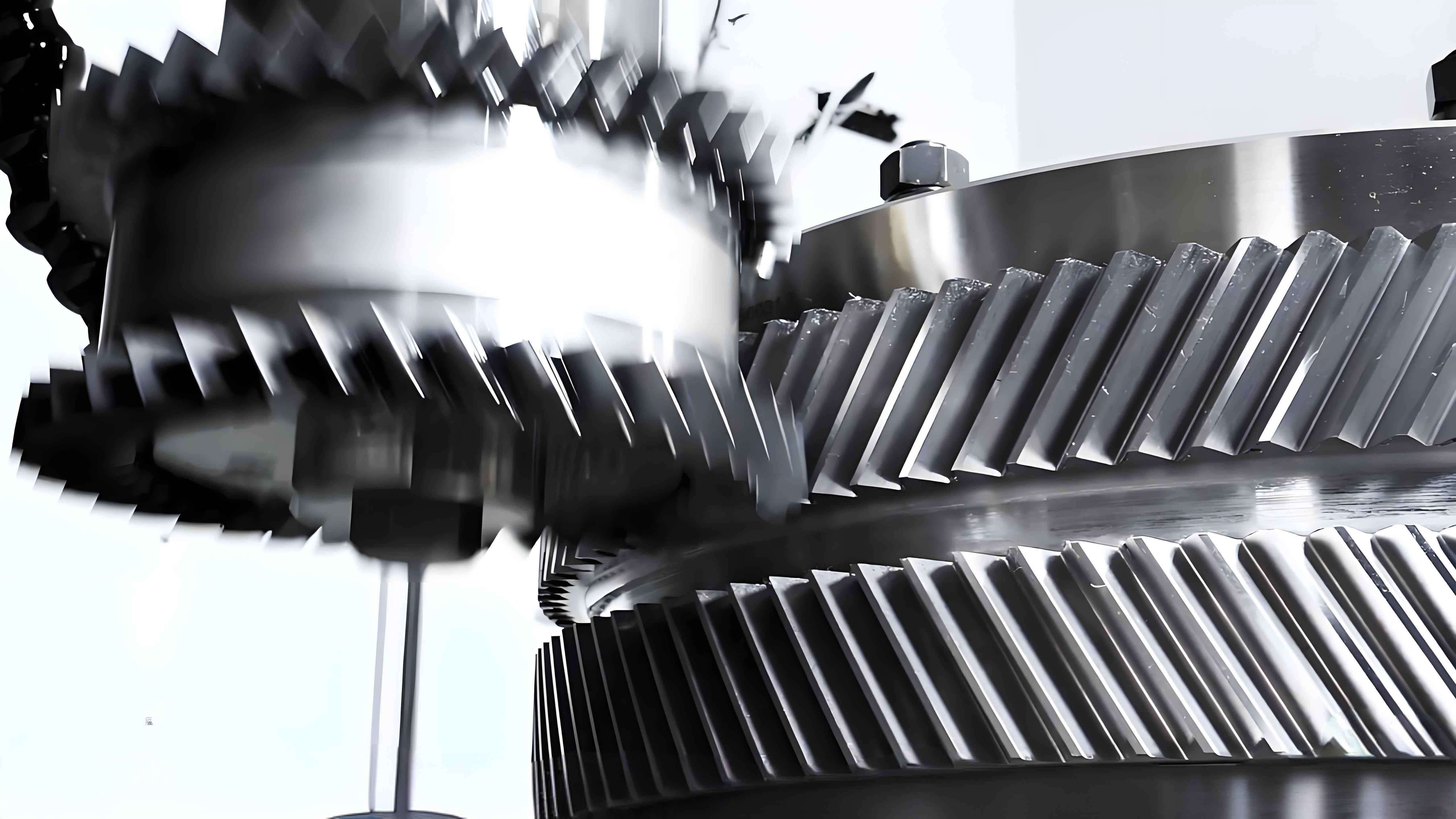
The derivation of narrow herringbone gear tooth surfaces starts with the concept of tooth profile evolution from traditional herringbone gears. Imagine a standard herringbone gear with left-hand and right-hand helical teeth; by reducing the groove width to zero and alternately extending and superimposing the tooth surfaces along the tooth width, we obtain the narrow herringbone gear configuration. This results in active gear teeth with alternating left-hand and right-hand profiles for the driving gear, and driven gear teeth with alternating left-hand and right-hand grooves, similar to variable-thickness gears. The tooth top cylinder and meshing start cylinder are straight cylindrical surfaces, and the involute tooth profile on the mid-end cross-section matches that of helical and herringbone gears. The calculation of tooth top radius, pitch radius, and root radius follows helical gear methods, though root radius calculation differs. We refer to the corresponding helical and herringbone gears with the same effective tooth width as equivalent helical gears and equivalent herringbone gears, respectively. During transmission, the left-hand and right-hand tooth surfaces alternately engage and disengage, resembling herringbone gear behavior when two pairs of teeth mesh simultaneously and helical gear behavior when only one pair meshes.
To mathematically describe the tooth surfaces, we use a generating rack method. Consider a rack surface that envelopes the narrow herringbone gear teeth. As the rack moves relative to the gear blanks with velocity \( v \), the gear blanks rotate with angular velocities \( \omega_1 \) and \( \omega_2 \). The upper side of the rack surface generates the driven gear, while the lower side generates the driving gear. The rack tooth surfaces are periodic every four faces, so we focus on a reference tooth surface for derivation. We establish coordinate systems: \( S_r (O_r – x_r y_r z_r) \) fixed to the rack, \( S_{rL} (O_{rL} – x_{rL} y_{rL} z_{rL}) \) for left-hand surfaces, and \( S_{rR} (O_{rR} – x_{rR} y_{rR} z_{rR}) \) for right-hand surfaces, all with the \( xz \)-plane on the pitch plane. The transformation between \( S_{rL} \) and \( S_r \) is given by:
$$ M_{rrL} = \begin{bmatrix} 1 & 0 & 0 & b \tan \beta \\ 0 & 1 & 0 & 0 \\ 0 & 0 & 1 & b \\ 0 & 0 & 0 & 1 \end{bmatrix} $$
where \( \beta \) is the helix angle of the equivalent herringbone gear, and \( b \) is a parameter along the tooth width. In \( S_{rL} \), the profile of the reference tooth surface in the \( x_{rL} y_{rL} \)-plane is:
$$ \mathbf{x}_{rL2} = \begin{bmatrix} -u \sin \alpha_t – \frac{p_t}{4} \\ u \cos \alpha_t \\ 0 \\ 1 \end{bmatrix} $$
where \( \alpha_t \) is the transverse pressure angle, \( p_t \) is the transverse pitch, and \( u \) is a parameter along the tooth height. Transforming to \( S_r \), the rack tooth surface equation becomes:
$$ \mathbf{R}_{r2} = M_{rrL} \mathbf{x}_{rL2} = \begin{bmatrix} -u \sin \alpha_t – \frac{p_t}{4} + b \tan \beta \\ u \cos \alpha_t \\ b \\ 1 \end{bmatrix} $$
For gear generation, we set up fixed coordinate system \( S (O – x y z) \), rack system \( S_r \), and gear systems \( S_1 (O_1 – x_1 y_1 z_1) \) for the driving gear and \( S_2 (O_2 – x_2 y_2 z_2) \) for the driven gear. The transformation matrices are:
$$ M_{1r} = \begin{bmatrix} \cos \psi_1 & \sin \psi_1 & 0 & -r_1 \psi_1 \cos \psi_1 + r_1 \sin \psi_1 \\ -\sin \psi_1 & \cos \psi_1 & 0 & r_1 \psi_1 \sin \psi_1 + r_1 \cos \psi_1 \\ 0 & 0 & 1 & 0 \\ 0 & 0 & 0 & 1 \end{bmatrix} $$
$$ M_{2r} = \begin{bmatrix} \cos \psi_2 & -\sin \psi_2 & 0 & -r_2 \psi_2 \cos \psi_2 + r_2 \sin \psi_2 \\ -\sin \psi_2 & -\cos \psi_2 & 0 & r_2 \psi_2 \sin \psi_2 + r_2 \cos \psi_2 \\ 0 & 0 & -1 & 0 \\ 0 & 0 & 0 & 1 \end{bmatrix} $$
where \( \psi_1 \) and \( \psi_2 \) are rotation angles, and \( r_1 \) and \( r_2 \) are pitch radii. The tooth surface family for the driving gear reference surface is:
$$ \mathbf{R}_{12} = M_{1r} \mathbf{R}_{r2} = \begin{bmatrix} \cos \psi_1 \left( -u \sin \alpha_t – \frac{p_t}{4} + b \tan \beta \right) + u \sin \psi_1 \cos \alpha_t – r_1 \psi_1 \cos \psi_1 + r_1 \sin \psi_1 \\ -\sin \psi_1 \left( -u \sin \alpha_t – \frac{p_t}{4} + b \tan \beta \right) + u \cos \psi_1 \cos \alpha_t + r_1 \psi_1 \sin \psi_1 + r_1 \cos \psi_1 \\ b \\ 1 \end{bmatrix} $$
and for the driven gear reference surface:
$$ \mathbf{R}_{22} = M_{2r} \mathbf{R}_{r2} = \begin{bmatrix} \cos \psi_2 \left( -u \sin \alpha_t – \frac{p_t}{4} + b \tan \beta \right) – u \sin \psi_2 \cos \alpha_t – r_2 \psi_2 \cos \psi_2 + r_2 \sin \psi_2 \\ -\sin \psi_2 \left( -u \sin \alpha_t – \frac{p_t}{4} + b \tan \beta \right) – u \cos \psi_2 \cos \alpha_t + r_2 \psi_2 \sin \psi_2 + r_2 \cos \psi_2 \\ -b \\ 1 \end{bmatrix} $$
The meshing condition requires that the normal vector \( \mathbf{n} \) and relative velocity \( \mathbf{v} \) satisfy \( \mathbf{n} \cdot \mathbf{v} = 0 \). The normal vector of the rack reference surface is:
$$ \mathbf{n} = \frac{\partial \mathbf{R}_{r2}}{\partial u} \times \frac{\partial \mathbf{R}_{r2}}{\partial b} = \cos \alpha_t \mathbf{i} + \sin \alpha_t \mathbf{j} + \tan \beta \cos \alpha_t \mathbf{k} $$
and the relative velocity for the driving gear is:
$$ \mathbf{v} = -\omega_1 u \cos \alpha_t \mathbf{i} + \omega_1 \left( -u \sin \alpha_t + r_1 \psi_1 – \frac{p_t}{4} + b \tan \beta \right) \mathbf{j} $$
Thus, the meshing equation for the driving gear is:
$$ f_{12}(u, b, \psi_1) = -u – \frac{p_t}{4} \sin \alpha_t + b \tan \beta \sin \alpha_t + r_1 \psi_1 \sin \alpha_t = 0 $$
and for the driven gear:
$$ f_{22}(u, b, \psi_2) = -u – \frac{p_t}{4} \sin \alpha_t + b \tan \beta \sin \alpha_t + r_2 \psi_2 \sin \alpha_t = 0 $$
The contact line equation on the rack surface at instant \( \psi_1^i \) (for \( i = 1, 2, \dots, n \)) is:
$$ \mathbf{R}_{r2} = x_{r2} \mathbf{i}_{r2} + y_{r2} \mathbf{j}_{r2} + z_{r2} \mathbf{k}_{r2}, \quad f_{12}(u, b, \psi_1^i) = 0 $$
which simplifies to:
$$ \begin{cases} x_{r2} = -u \sin \alpha_t – \frac{p_t}{4} + b \tan \beta \\ y_{r2} = u \cos \alpha_t \\ z_{r2} = b \\ -u – \frac{p_t}{4} \sin \alpha_t + b \tan \beta \sin \alpha_t + r_1 \psi_1 \sin \alpha_t = 0 \end{cases} $$
The meshing surface equation in the fixed coordinate system \( S \) is:
$$ \mathbf{R}_{0r} = M_{0r} \mathbf{R}_{r2}, \quad f_{12}(u, b, \psi_1) = 0 $$
with transformation matrix:
$$ M_{0r} = \begin{bmatrix} 1 & 0 & 0 & -r_1 \psi_1 \\ 0 & 1 & 0 & 0 \\ 0 & 0 & 1 & b \\ 0 & 0 & 0 & 1 \end{bmatrix} $$
yielding:
$$ \begin{cases} x_{0r} = -u \sin \alpha_t – \frac{p_t}{4} + b \tan \beta – r_1 \psi_1 \\ y_{0r} = u \cos \alpha_t \\ z_{0r} = b \\ -u – \frac{p_t}{4} \sin \alpha_t + b \tan \beta \sin \alpha_t + r_1 \psi_1 \sin \alpha_t = 0 \end{cases} $$
These equations form the basis for analyzing narrow herringbone gears. To validate and explore their meshing behavior, we proceed to model building and simulation. The parameters for narrow herringbone gears are similar to those of equivalent helical gears, but with even tooth numbers due to the four-face periodicity. The normal module \( m_n \) is used, and the transverse module is \( m_t = m_n / \cos \beta \). A condition to prevent tooth tip sharpening on the driven gear is:
$$ S’_a = -B \frac{z_2 + 2}{z_2} \tan \beta + m_t (z_2 + 2) \left( \frac{\pi}{2} \frac{1}{z_2} – (\tan \alpha_a – \alpha_a – \tan \alpha_t + \alpha_t) \right) > 0 $$
where \( S’_a \) is the tooth tip thickness, \( B \) is the face width, \( z_2 \) is the number of teeth on the driven gear, and \( \alpha_a \) is the pressure angle at the tooth tip. We define two example cases for analysis, as summarized in Table 1.
| Example | \( z_1 \) | \( z_2 \) | \( m_n \) (mm) | \( \alpha_n \) (°) | \( \beta \) (°) | \( B \) (mm) |
|---|---|---|---|---|---|---|
| Example 1 | 50 | 100 | 1.75 | 20 | 10 | 7 |
| Example 2 | 18 | 36 | 1.75 | 20 | 10 | 7 |
Using MATLAB, we compute the 3D coordinates of tooth surfaces based on the derived equations and generate point clouds. These are imported into UG to create precise solid models via surface fitting. The driving gear has alternating left-hand and right-hand tooth profiles, while the driven gear has alternating grooves. Interference checks in UG’s motion simulation module confirm model accuracy, with zero-volume interference surfaces indicating no clashes during meshing. This validates the correctness of our tooth surface equations and modeling approach for herringbone gears.
Next, we analyze the contact lines. The instantaneous contact lines are straight lines on the planar meshing surface. Using MATLAB, we calculate contact lines at various rotation angles of the driving gear: \( \psi_1 = [-5.44^\circ, -4.54^\circ, -1.84^\circ, 1.76^\circ, 5.36^\circ, 7.96^\circ, 8.86^\circ] \). The results show that left-hand and right-hand contact lines alternate as the gear rotates, with each tooth engaging from one end to the other, similar to helical gears. The total length of contact lines varies periodically, influencing the meshing stiffness and load distribution. For Example 1, the contact ratio \( \epsilon \) is 2.00, meaning there is no single-tooth contact region but single-tooth contact points at \( \psi_1 = -5.5^\circ, 1.6^\circ, 8.7^\circ \). For Example 2, \( \epsilon = 1.82 \), so a single-tooth contact region exists. Compared to equivalent herringbone gears, narrow herringbone gears have higher contact ratios because they use the full face width without a groove, enhancing the longitudinal contact ratio \( \epsilon_\beta = B \tan \beta / (\pi m_t) \). The equivalent herringbone gears for Examples 1 and 2 have contact ratios of 1.89 and 1.71, respectively. This demonstrates the advantage of narrow herringbone gears in improving meshing continuity.
To quantify contact line behavior, we compute the total contact line length over a meshing cycle. Under ideal conditions, load is uniformly distributed along the contact lines. For a constant load transmission, the force density \( q \) changes with contact line length. When both left-hand and right-hand tooth surfaces are engaged, axial forces partially cancel. The net axial force \( F_a \) depends on the difference between left-hand contact length \( l_l \) and right-hand contact length \( l_r \), given by \( F_a = q (l_l – l_r) \sin \beta_b \), where \( \beta_b \) is the base helix angle. Radial force \( F_r \) and tangential force \( F_t \) remain constant. Using the parameters from Table 1 with a load torque of 100 N·m, we calculate theoretical axial forces and compare them with ADAMS simulation results. The data are summarized in Table 2.
| Gear Type | \( \epsilon \) | \( F_r \) (N) | \( F_t \) (N) | \( F_a \) (N) |
|---|---|---|---|---|
| Narrow Herringbone Gear (Example 1) | 2.00 | 430 | 1160 | < 60 |
| Equivalent Helical Gear | 2.00 | 430 | 1160 | 200 |
| Equivalent Herringbone Gear | 1.89 | 430 | 1160 | 0 |
| Narrow Herringbone Gear (Example 2) | 1.82 | 1230 | 3320 | < 300 |
| Equivalent Helical Gear | 1.82 | 1230 | 3320 | 570 |
| Equivalent Herringbone Gear | 1.71 | 1230 | 3320 | 0 |
The theoretical axial force for narrow herringbone gears fluctuates, peaking when the difference in left-hand and right-hand contact lengths is maximal. For Example 1, fluctuations are small because the contact ratio is 2, ensuring at least two teeth are in contact, reducing axial force variation. In contrast, Example 2 shows larger fluctuations due to the lower contact ratio. ADAMS simulations corroborate these trends, though with smaller amplitudes due to practical factors like damping and flexibility. As the contact ratio increases, axial force fluctuations diminish, approaching zero like in traditional herringbone gears. This highlights the balance narrow herringbone gears strike between helical and herringbone gear characteristics.
Further insights come from examining the contact line length variations. For Example 1, the total contact line length changes cyclically, with minima at single-tooth contact points and maxima during double-tooth engagement. The contact ratio calculation confirms this pattern: \( \epsilon = \epsilon_\alpha + \epsilon_\beta \), where \( \epsilon_\alpha \) is the transverse contact ratio and \( \epsilon_\beta \) is the longitudinal contact ratio. For narrow herringbone gears, \( \epsilon_\beta \) is maximized due to the full face width utilization. We can express the contact line length \( L \) as a function of rotation angle \( \psi_1 \):
$$ L(\psi_1) = \sum_{i=1}^{n} l_i(\psi_1) $$
where \( l_i \) is the length of the \( i \)-th contact line, derived from the meshing equations. Using MATLAB, we plot \( L(\psi_1) \) over a meshing cycle, showing periodic peaks and troughs. This variability affects the dynamic response and noise generation, areas where herringbone gears traditionally excel. By optimizing parameters like helix angle and face width, we can tailor narrow herringbone gears for specific applications, such as high-speed transmissions or heavy-load machinery.
In terms of manufacturing, narrow herringbone gears pose challenges due to their alternating tooth surfaces. However, advanced methods like CNC grinding or hobbling can be adapted, building on techniques used for herringbone gears. The elimination of a groove simplifies tooling to some extent, but precise control of tooth thickness variation is required. Future work could explore additive manufacturing for prototyping these gears. Additionally, tooth profile modifications, common in herringbone gears to reduce vibration and noise, can be applied to narrow herringbone gears. For instance, tip and root relief or lead crowning could enhance performance, as studied in traditional herringbone gear optimizations.
From a design perspective, narrow herringbone gears offer flexibility in gearbox layout. Their compact width-diameter ratio allows for smaller housing sizes, beneficial in aerospace or automotive applications. The axial force reduction minimizes bearing loads, extending component life. Moreover, the variable-thickness nature of the driven gear can compensate for assembly errors or thermal expansion, improving reliability. These advantages make narrow herringbone gears a promising alternative in the family of herringbone gears, especially where space and weight constraints are critical.
To deepen the analysis, we consider the stress distribution on tooth surfaces. Using finite element analysis (FEA) in conjunction with UG models, we can simulate contact stresses under load. The Hertzian contact theory provides a baseline, but for herringbone-like gears, the alternating engagement complicates stress patterns. The maximum contact stress \( \sigma_H \) can be estimated using:
$$ \sigma_H = \sqrt{ \frac{F_t}{b \rho_r} \cdot \frac{1}{\pi \left( \frac{1-\nu_1^2}{E_1} + \frac{1-\nu_2^2}{E_2} \right)} } $$
where \( \rho_r \) is the relative curvature radius, \( b \) is the face width, \( E \) is Young’s modulus, and \( \nu \) is Poisson’s ratio. For narrow herringbone gears, the effective face width varies along the tooth, so average values or localized analysis may be needed. FEA results could be tabulated to compare stress levels with equivalent gears, but that extends beyond this article’s scope.
In conclusion, our exploration of narrow herringbone gears reveals their unique meshing and force characteristics. Derived from traditional herringbone gears, they feature alternately arranged left-hand and right-hand tooth surfaces, eliminating grooves and increasing contact ratios. The tooth surface equations, derived via a generating rack method, enable precise modeling and interference-free operation. Contact line analysis shows alternating patterns akin to helical gears, with total length fluctuations influencing axial forces. Force analysis demonstrates that axial forces are lower than in equivalent helical gears and fluctuate with an amplitude that decreases as contact ratio increases. This makes narrow herringbone gears suitable for applications requiring reduced axial load and compact design, filling a niche between helical and herringbone gears. Future research could focus on dynamic modeling, noise reduction, and manufacturing techniques to further harness the potential of herringbone gears in modern machinery.
Throughout this study, we have emphasized the importance of herringbone gears in mechanical transmission systems. The narrow herringbone gear variant builds on this legacy, offering improved performance metrics. By integrating mathematical modeling, software simulation, and theoretical analysis, we provide a comprehensive framework for understanding and designing these gears. As technology advances, innovations like narrow herringbone gears will continue to evolve, pushing the boundaries of gear transmission efficiency and reliability.