
Spiral bevel gears are indispensable components in aerospace and automotive powertrains, prized for their high load capacity, smooth operation, and superior power transmission efficiency for intersecting shafts. These advantages stem from their curved teeth, which enable gradual engagement and higher contact ratios compared to straight bevel gears. However, the very design that grants these benefits—often featuring a thin, disk-like web or blank for weight reduction—makes them susceptible to high-cycle fatigue failures under demanding operational conditions characterized by high speeds, elevated temperatures, and significant alternating loads. A primary failure mechanism in such thin-rimmed, high-speed spiral bevel gears is traveling wave resonance, a destructive phenomenon where standing wave patterns (characterized by nodal diameters) rotate relative to the gear, leading to excessive dynamic stresses, particularly at the tooth root fillets on the gear’s back face. Predicting and mitigating this resonance is therefore a critical aspect of ensuring the structural integrity and reliability of modern transmission systems. This article presents a detailed, system-level methodology for the analysis and prediction of traveling wave resonance in spiral bevel gears, encompassing precise geometric modeling, prestressed modal analysis, resonance speed prediction, and experimental validation.
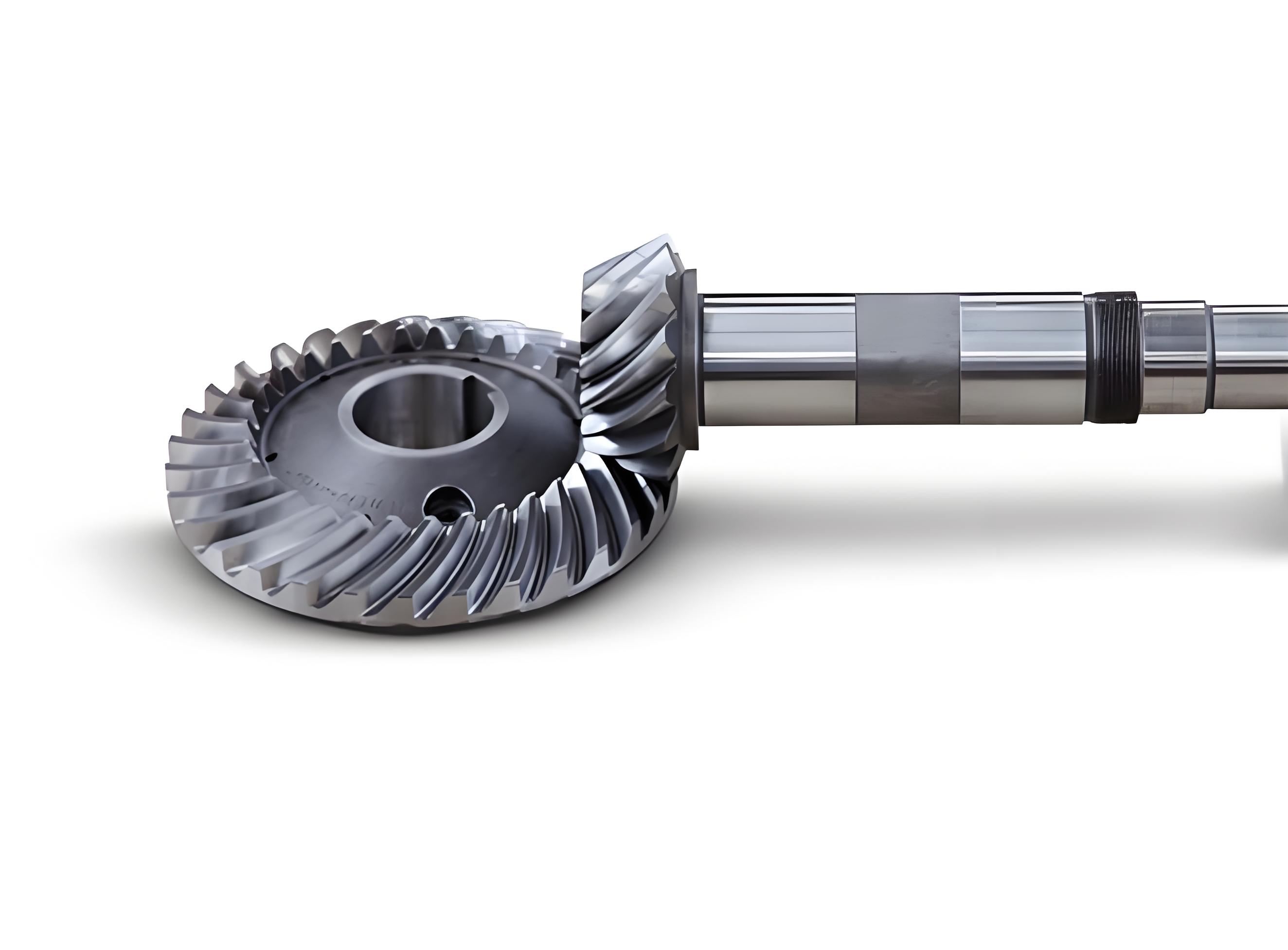
The accurate prediction of dynamic behavior, especially resonant frequencies and modes, hinges on the fidelity of the computational model. A significant challenge lies in moving beyond simplified macro-geometric models to incorporate the exact tooth surface geometry, which is defined by a complex interplay of design parameters and manufacturing settings (machine tool settings, cutter geometry, etc.). The contact conditions and load distribution between mating spiral bevel gears are highly sensitive to these micro-geometries. An imprecise model can lead to erroneous contact patterns and stress distributions, which in turn affect the calculated system stiffness and, consequently, the predicted natural frequencies. This work addresses this challenge by initiating the analysis with the creation of a three-dimensional finite element model based on exact tooth surface data derived from both design and manufacturing parameters. Subsequently, a static analysis is performed to establish proper contact under load, followed by a prestressed modal analysis to extract the system’s natural frequencies and mode shapes. These modal characteristics are then used in conjunction with traveling wave resonance theory to predict critical speeds within the operational range. Finally, the entire predictive methodology is rigorously validated against experimental data obtained from a dedicated test rig, confirming its accuracy and practical utility for design evaluation and resonance avoidance in spiral bevel gear systems.
Methodology for System-Level Analysis
The proposed methodology is a sequential, integrated process designed to capture the critical physics governing the traveling wave resonance of spiral bevel gear systems. It consists of four primary stages: 1) Generation of a high-fidelity 3D Finite Element Model (FEM) with exact tooth geometry, 2) System-level modeling incorporating supports and contacts, 3) Prestressed modal analysis to obtain dynamic characteristics, and 4) Traveling wave resonance prediction and experimental correlation.
Stage 1: Generation of High-Fidelity Gear Pair Model
The foundation of any reliable dynamic analysis is an accurate geometric representation. For spiral bevel gears, the tooth flank is a complex, non-developable surface generated by a relative rolling motion between the gear blank and a hypothetical crown gear or via specific machine tool kinematics. The final surface geometry is not solely defined by basic design parameters (module, number of teeth, spiral angle) but is critically influenced by manufacturing or machine settings (cutter radius, tilt angle, machine root angle, etc.). Therefore, the modeling process begins by utilizing dedicated gear design software (e.g., MASTA, KISSsoft, or specialized in-house codes). The macro-parameters, such as those listed in Table 1, are first input to define the gear blank and basic gear geometry.
| Parameter | Pinion | Gear |
|---|---|---|
| Number of Teeth | 40 | 41 |
| Module (mm) | 3.24 | 3.24 |
| Mean Spiral Angle (°) | 35 | 35 |
| Normal Pressure Angle (°) | 20 | 20 |
| Shaft Angle (°) | 80 | |
| Face Width (mm) | 26 | |
| Hand of Spiral | Right Hand | Left Hand |
Subsequently, the detailed manufacturing parameters for both the gear and the pinion (concave and convex flanks separately) are entered into the software’s manufacturing simulation module. These parameters, exemplified in Table 2 for the gear member, control the detailed form of the tooth, including profile and lengthwise crowning, bias, and flank twist. The software then calculates the coordinates of points defining the exact tooth surface, typically organized in a grid (e.g., 7 points along the profile and 9 points along the length). This point cloud data for all flanks is exported.
| Parameter | Value |
|---|---|
| Blank Tilt Angle (°) | 62.3772 |
| Machine Center to Crossing Point (mm) | 0 |
| Cutter Radius (mm) | 82.156 |
| Ratio of Roll | 1.5342 |
| Swivel Angle (°) | 207.36 |
| Inside Blade Angle (°) | 21 |
| Inside Tip Radius (mm) | 0.65 |
This exported data forms the basis for building the solid model. Using CAD software (e.g., CATIA, NX, or SolidWorks), the point clouds are imported. Spline curves are constructed through these points along constant profile and lengthwise lines. These splines are then used to generate a network of surfaces, which are stitched together to form a single, continuous tooth flank surface. This surface is then used to trim the basic gear blank, creating one precise tooth. This tooth is then patterned circumferentially to complete the full gear or pinion model. This process ensures that the FEM geometry reflects the as-manufactured tooth form, including all intentional modifications, which is crucial for accurate contact analysis.
Stage 2: System-Level Finite Element Modeling
The dynamic behavior of the gears cannot be analyzed in isolation; it is a function of the entire system, including shafts, bearings, and housing. Therefore, a system-level model is constructed. The precisely modeled pinion and gear are assembled onto their respective shafts. The shaft geometry, including any features like shoulders and splines, is modeled in detail. The material properties for all steel components (gears and shafts) are assigned: Young’s Modulus $$E = 204 \text{ GPa}$$, Density $$\rho = 7850 \text{ kg/m}^3$$, and Poisson’s ratio $$\nu = 0.293$$.
The connection between the mating tooth flanks is modeled using a surface-to-surface frictional contact formulation. A friction coefficient of $$\mu = 0.1$$ is typically assumed. The supports provided by the bearings are critical boundary conditions. Instead of modeling the bearings and housing explicitly, which would drastically increase model complexity, their effect is simulated using linear spring elements (CBUSH or similar elements in FEA software) attached to the shaft at the bearing locations. These springs represent the translational stiffness of the bearing-housing combination in the radial (X, Y) and axial (Z) directions. The stiffness values, often obtained from bearing catalogs or dedicated housing analysis, are applied as shown in Table 3. This approach captures the essential flexibility of the support structure efficiently.
| Bearing Location | Kx (N/mm) | Ky (N/mm) | Kz (N/mm) |
|---|---|---|---|
| A | 319,550 | 319,550 | 1 |
| B | 69,973 | 69,973 | 34,243 |
| C | 338,250 | 338,250 | 1 |
| D | 448,380 | 448,380 | 1 |
| E | 307,540 | 307,540 | 1 |
| F | 262,930 | 262,930 | 139,850 |
Stage 3: Prestressed Modal Analysis
Standard modal analysis assumes linear elastic behavior and small deformations from an unloaded state. For a gear pair, this is unrealistic because the gears are in constant contact under load during operation. The contact pressure and the resulting mesh stiffness significantly influence the system’s dynamic characteristics. A prestressed modal analysis addresses this by being a two-step procedure:
Step 1: Nonlinear Static Analysis. A static torque is applied to the input shaft (e.g., $$T = 100 \text{ Nm}$$), and a rotational constraint is applied to the output shaft. This analysis solves for the equilibrium state, including contact penetration, friction, and the resulting stress field. The outcome verifies that the contact pattern (ellipse) is correctly located on the tooth flank and that the contact pressure is within acceptable limits, ensuring the model is behaving physically correct under load.
Step 2: Linear Perturbation Modal Analysis. The stressed state from the static analysis (including the stiffness from the established contact regions) is used as the initial condition for an eigenvalue extraction. The software linearizes the system around this prestressed state and calculates the natural frequencies and corresponding mode shapes. This method yields modal properties that are representative of the gears’ operating condition, making them far more accurate for resonance prediction than modes from an unloaded model or one with tied contacts.
Stage 4: Traveling Wave Resonance Theory and Prediction
For a stationary, disk-like structure such as a gear web, a lateral bending vibration mode with *m* nodal diameters can be described as a standing wave. Its displacement *z* can be expressed as a function of radial position *r*, angular position $$\theta$$, and time *t*:
$$ z = A(r) \cos(m\theta) \cos(\omega_d t) $$
where $$A(r)$$ is the radial amplitude function, and $$\omega_d$$ is the natural frequency (in rad/s) of the standing wave, also called the *dynamical frequency*.
When this gear rotates at a speed $$\Omega$$ (in rad/s, or $$n$$ in RPM where $$\Omega = 2\pi n / 60$$), an observer in the fixed frame perceives this standing wave as the sum of two traveling waves rotating in opposite directions:
$$ z = \frac{1}{2}A(r) \left[ \cos(m\theta – \omega_d t) + \cos(m\theta + \omega_d t) \right] $$
These are the *forward* and *backward* traveling waves, with frequencies $$f_f$$ and $$f_b$$ (in Hz) given by:
$$ f_f = f_d + \frac{z_1}{z_2} \cdot \frac{n \cdot m}{60} $$
$$ f_b = f_d – \frac{z_1}{z_2} \cdot \frac{n \cdot m}{60} $$
Here, $$f_d = \omega_d / 2\pi$$ is the dynamical frequency in Hz, $$z_1$$ and $$z_2$$ are the numbers of teeth on the pinion and gear, and $$n$$ is the rotational speed of the pinion in RPM. The term $$\frac{z_1}{z_2} \cdot n$$ is the rotational speed of the gear.
The primary excitation in a gear mesh is at the tooth meshing frequency $$f_e$$:
$$ f_e = \frac{n}{60} \cdot z_1 $$
Resonance occurs when this excitation frequency coincides with the frequency of a traveling wave in the fixed frame. Therefore, the critical speeds $$n_{crit}$$ for resonance are found by setting $$f_e = f_f$$ or $$f_e = f_b$$ and solving for $$n$$:
$$ n_{crit} = \frac{60 \cdot f_d}{z_1 \left( \frac{z_2 \mp m}{z_2} \right)} = \frac{60 \cdot f_d}{z_1 \mp m \cdot \left( \frac{z_1}{z_2} \right) } $$
The minus sign corresponds to forward wave resonance, and the plus sign to backward wave resonance. By extracting the dynamical frequencies $$f_d$$ for various *m*-nodal-diameter modes from the prestressed modal analysis, one can construct a Campbell diagram. This diagram plots the system’s natural frequencies and the excitation frequencies (mesh frequency and its harmonics) against the rotational speed. The intersection points between the excitation lines and the frequency lines (which are horizontal for the standing wave frequency but split into two slopes for the traveling waves in a rotating frame) indicate the predicted critical speeds for traveling wave resonance.
Analysis Results and Discussion
The described methodology was applied to a specific aero-engine spiral bevel gear system test article. The prestressed modal analysis yielded a comprehensive set of natural frequencies and mode shapes up to 22 kHz. A subset of the most relevant modes, primarily those involving disk-type bending of the pinion and gear webs, is summarized in Table 4. The results reveal several important characteristics of the system’s dynamics.
| Mode Order | Frequency (Hz) | Dominant Mode Shape Description |
|---|---|---|
| 1 | 3,074.7 | Coupled 1-nodal-diameter (Pinion & Gear) |
| 3 | 3,493.2 | 1-nodal-diameter (Primarily Pinion) |
| 5 | 4,540.1 | 2-nodal-diameter (Pinion) |
| 7 | 4,776.4 | 2-nodal-diameter (Gear) |
| 9 | 7,225.0 | Umbrella (Conical) Mode (Pinion) |
| 11 | 9,594.8 | 3-nodal-diameter (Gear) |
| 12 | 9,612.9 | 3-nodal-diameter (Pinion) |
| 17 | 15,881 | 4-nodal-diameter (Gear) |
| 19 | 16,020 | 4-nodal-diameter (Pinion) |
A key observation is the presence of closely spaced frequencies for similar mode shapes on the pinion and gear. For instance, the 2-nodal-diameter modes of the pinion and gear (Modes 5 and 7) are separated by only 236 Hz, and the 3-nodal-diameter modes (Modes 11 and 12) are separated by a mere 18 Hz. This indicates strong dynamic coupling in the system or similar individual component stiffness/mass properties. The modal sequence is logically ordered: 1-nodal-diameter modes appear first (lowest frequency), followed by 2-nodal-diameter, then umbrella modes, then 3-nodal-diameter, and finally 4-nodal-diameter modes. This clear separation is beneficial for mode identification but can pose a challenge for frequency tuning, as shifting one frequency might inadvertently bring another into resonance.
Using the frequencies from Table 4 and the governing equations for traveling wave resonance, a Campbell diagram was constructed for the operational speed range of 0 to 16,000 RPM (pinion input). The intersections of the mesh frequency line $$f_e = n \cdot z_1 / 60$$ with the forward/backward traveling wave frequency lines for each mode yield the predicted critical speeds. A consolidated list of predicted resonance speeds for the most significant modes is presented in Table 5.
| Resonance Type | Predicted Speed Range (RPM) | Corresponding Dynamical Frequency f_d (Hz) |
|---|---|---|
| 1-Nodal-Diameter (System) | 4,117 – 6,043 | ~3,074 – 4,293 |
| 2-Nodal-Diameter (Primarily) | 6,060 – 7,828 | ~4,540 – 5,418 |
| 3-Nodal-Diameter (Primarily) | 12,270 – 14,754 | ~9,594 – 9,944 |
| 4-Nodal-Diameter (Primarily) | 15,093 – 16,154 | ~11,548 – 16,154 |
Experimental Validation and Correlation
To validate the analytical predictions, a dedicated test was conducted on a gearbox test rig housing the physical spiral bevel gear system. Tri-axial accelerometers were mounted on the bearing housings of both the input and output shafts to capture vibration responses. The test involved a slow ramp-up of the input shaft speed from 0 to 16,000 RPM under a constant output torque load of approximately 30 Nm, while continuously recording vibration data.
The analysis of the experimental data focused on the root mean square (RMS) value of vibration acceleration as a function of speed. Distinct resonance peaks and speed ranges with elevated vibration were identified. The primary experimental resonance intervals are summarized in Table 6 and compared directly with the theoretical predictions.
| Theoretical Prediction | Experimental Result | Agreement & Remarks |
|---|---|---|
| 1-ND Range: 4,117 – 6,043 RPM | No distinct peak observed | Poor. Likely due to model boundary condition discrepancies affecting this highly system-dependent mode, or low excitation/response at sensor locations. |
| 2-ND Range: 6,060 – 7,828 RPM | Strong peak at ~6,002 RPM and elevated vibration from 6,836 – 7,896 RPM | Excellent. The predicted onset (6,060 RPM) and range correlate very well with the measured major peak (6,002 RPM, -0.96% error) and the sustained high-vibration zone. |
| 3-ND Range: 12,270 – 14,754 RPM | Elevated vibration from 12,270 – 14,360 RPM | Excellent. The predicted lower bound matches exactly (12,270 RPM). The upper bound prediction (14,754 RPM) is within 2.74% of the measured zone end (14,360 RPM). |
The correlation between the predicted and experimental results for the 2-nodal-diameter and 3-nodal-diameter resonances is remarkably strong, with speed errors of less than 2.74%. This high degree of accuracy validates the core of the proposed methodology: the use of a precise geometric model combined with a prestressed system-level modal analysis for predicting traveling wave resonance in spiral bevel gears. The absence of a clear 1-nodal-diameter resonance in the test data is not uncommon. First-nodal-diameter modes are often heavily damped by the system (bearings, oil) and can be highly sensitive to the exact boundary conditions, which are difficult to replicate perfectly in the FEM with linear spring supports. Furthermore, the excitation force vector or the response measurement location might not optimally couple with this particular mode shape.
Conclusion
This work has successfully developed and demonstrated a comprehensive, system-level methodology for analyzing and predicting traveling wave resonance in high-speed spiral bevel gear systems. The methodology’s strength lies in its integrated approach, starting from the generation of a geometrically precise finite element model based on manufacturing data, progressing through a system-level static and prestressed modal analysis to capture operational dynamic characteristics, and culminating in the application of traveling wave resonance theory to predict critical speeds.
The key findings and contributions are:
- The necessity of precise tooth flank modeling for accurate dynamic system representation is confirmed. The contact-induced stiffness from the static analysis significantly influences the modal frequencies.
- The prestressed modal analysis provides a realistic set of natural frequencies and mode shapes that account for the loaded state of the gear mesh, which is essential for resonance prediction in operating conditions.
- The theoretical predictions for the 2-nodal-diameter and 3-nodal-diameter traveling wave resonances showed excellent agreement with experimental data, with errors in critical speed prediction of less than 3%. This validates the predictive capability of the methodology for the most critical resonance modes typically responsible for high-cycle fatigue failures in spiral bevel gears.
- The methodology provides a valuable, practical engineering tool. It enables designers to identify potential resonance risks during the design phase. Based on the predictions, corrective actions can be taken, such as:
- Structural modification (e.g., changing web thickness, adding stiffening ribs) to shift natural frequencies.
- Implementing damping solutions (e.g., constrained layer dampers, tuned mass dampers) within the gear design.
- Establishing operational procedures that require “fast passage” through identified critical speed ranges during run-up or run-down sequences in engine testing.
Future work could focus on incorporating more sophisticated damping models into the analysis, extending the methodology to include the effects of multiple harmonic excitations, and investigating the sensitivity of the results to variations in key parameters such as bearing stiffness and assembly misalignment. Nevertheless, the presented approach offers a robust and validated framework for ensuring the dynamic integrity and reliability of spiral bevel gear systems in demanding applications.