
In my research on the manufacturing of hypoid bevel gear drives, I treat the tooth surface as the central link between design intent, numerical control machining, measurement, and final transmission behavior. A hypoid bevel gear is not a simple geometric object. Its flank is generated by a complex relative motion between a cutter head and a workpiece, and the resulting surface is sensitive to machine settings, cutter geometry, thermal distortion, fixture error, and measurement uncertainty. For commercial vehicle drive axles, the hypoid bevel gear transmits torque with a large reduction ratio, a high contact ratio, and a small package envelope. Therefore, the accuracy of the hypoid bevel gear tooth surface directly influences vibration, noise, fatigue life, and overall driveline quality.
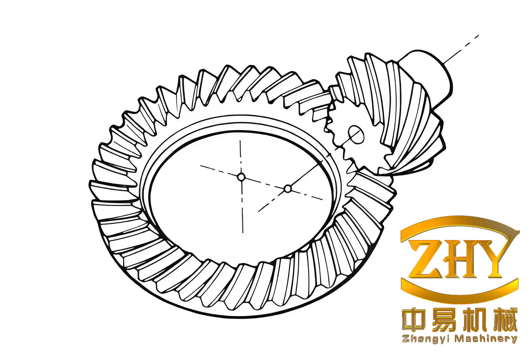
In my first-person account, I start from the mathematical modeling of the hypoid bevel gear tooth surface. I then build a five-axis numerical control machining simulation platform, study the influence of machine adjustment parameters on tooth surface error, propose an improved linear regression method for correcting that error, and validate the method through measurement and correction experiments. Throughout this work, I use the term hypoid bevel gear repeatedly because every modeling step, every simulation decision, and every correction strategy is ultimately aimed at improving the hypoid bevel gear tooth surface.
The core problem can be stated as follows. A theoretical hypoid bevel gear tooth surface is defined by a set of machine adjustment parameters and cutter parameters. In actual production, the manufactured hypoid bevel gear tooth surface deviates from the theoretical surface. The deviation is not random in a geometric sense; it is a systematic mapping of parameter errors into normal-direction tooth surface error. If I can identify a sensitivity relationship between the machine adjustment parameters and the tooth surface error, I can invert that relationship and compute correction amounts for the machine adjustment parameters. The difficulty is that the sensitivity matrix is often ill-conditioned, the number of correction parameters may be large, and the correction must remain practical on a real machine tool. My improved method addresses this difficulty by selecting the most effective correction parameters while keeping the number of corrected parameters as small as possible.
To make the mathematical treatment clear, I define the theoretical hypoid bevel gear tooth surface as a vector function of two surface parameters and a set of machine settings. I write the general form as
$$ \mathbf{r} = \mathbf{r}(s,\theta,\phi,k) $$
where \(s\) is the cutting depth along the blade, \(\theta\) is the cutter phase angle, \(\phi\) is the workpiece rotation angle, and \(k\) is the vector of machine adjustment parameters. For the hypoid bevel gear, \(k\) may include the tilt angle, swivel angle, radial cutter position, initial cradle angle, vertical offset,床位, horizontal offset, machine root angle, and roll ratio. In my notation, I keep the mathematical symbols consistent across the gear and pinion because the same coordinate transformation logic applies to both members of the hypoid bevel gear pair.
The cutter head is the origin of the tooth surface geometry. For a face-milling cutter, the cutting edge is modeled as a conical surface. In the cutter coordinate system, a point on the cutting edge is
$$ \mathbf{r}_c(s,\theta)= \begin{bmatrix} (R \mp s \sin \alpha)\cos\theta \\ (R \mp s \sin \alpha)\sin\theta \\ -s\cos\alpha \\ 1 \end{bmatrix} $$
where \(R\) is the tip radius, \(\alpha\) is the blade profile angle, and the upper sign corresponds to the inside blade while the lower sign corresponds to the outside blade. The unit normal of the cutter surface is obtained from the cross product of the partial derivatives:
$$ \mathbf{n}_c(\theta)=\frac{\mathbf{N}_c}{\|\mathbf{N}_c\|}, \qquad \mathbf{N}_c=\frac{\partial \mathbf{r}_c}{\partial s}\times\frac{\partial \mathbf{r}_c}{\partial \theta} $$
For the cutter head, this becomes
$$ \mathbf{n}_c(\theta)= \begin{bmatrix} \cos\alpha\cos\theta \\ \cos\alpha\sin\theta \\ \mp \sin\alpha \end{bmatrix} $$
I use these cutter equations as the foundation for both the formate gear tooth surface and the tilt-generated pinion tooth surface. The hypoid bevel gear pair in a drive axle usually has a formate gear and a generated pinion. The formate gear is simpler because the cradle does not roll during the final cut. The generated pinion is more complex because the cutter tilt and swivel mechanisms create a conical generating wheel, and the pinion tooth surface is obtained through the meshing equation.
For the formate gear, I establish a cutter coordinate system, a machine fixed coordinate system, and a gear blank coordinate system. The transformation from the cutter system to the machine system is
$$ M_{mc}= \begin{bmatrix} 1 & 0 & 0 & H \\ 0 & 1 & 0 & V \\ 0 & 0 & 1 & -\Delta B_1 \\ 0 & 0 & 0 & 1 \end{bmatrix} $$
and the transformation from the machine system to the gear blank system is
$$ M_{1m}= \begin{bmatrix} \cos\gamma_{m1} & 0 & \sin\gamma_{m1} & -\Delta A_1 \\ 0 & 1 & 0 & 0 \\ -\sin\gamma_{m1} & 0 & \cos\gamma_{m1} & 0 \\ 0 & 0 & 0 & 1 \end{bmatrix} $$
Therefore, the formate gear tooth surface and its normal are
$$ \mathbf{r}_1(s_1,\theta_1)=M_{1m}M_{mc}\mathbf{r}_c(s_1,\theta_1) $$
$$ \mathbf{n}_1(\theta_1)=M_{1m}M_{mc}\mathbf{n}_c(\theta_1) $$
For the generated pinion, I introduce the cutter tilt coordinate system, the cutter swivel coordinate system, the cradle coordinate system, the machine center coordinate system, the workhead coordinate system, and the pinion blank coordinate system. The chain of transformations is long, but it is necessary because the hypoid bevel gear pinion tooth surface is created by the relative motion between the generating wheel and the pinion blank. I write the main matrices as
$$ M_{ac}= \begin{bmatrix} \cos i & 0 & \sin i & 0 \\ 0 & 1 & 0 & 0 \\ -\sin i & 0 & \cos i & 0 \\ 0 & 0 & 0 & 1 \end{bmatrix} $$
$$ M_{ba}= \begin{bmatrix} -\sin j & -\cos j & 0 & S_R \\ \cos j & -\sin j & 0 & 0 \\ 0 & 0 & 1 & 0 \\ 0 & 0 & 0 & 1 \end{bmatrix} $$
$$ M_{db}= \begin{bmatrix} \cos q & \pm \sin q & 0 & 0 \\ \mp \sin q & \cos q & 0 & 0 \\ 0 & 0 & 1 & 0 \\ 0 & 0 & 0 & 1 \end{bmatrix} $$
$$ M_{ed}= \begin{bmatrix} 1 & 0 & 0 & 0 \\ 0 & 1 & 0 & E_m \\ 0 & 0 & 1 & -\Delta B_2 \\ 0 & 0 & 0 & 1 \end{bmatrix} $$
$$ M_{fe}= \begin{bmatrix} \cos\gamma_{m2} & 0 & \sin\gamma_{m2} & -\Delta A_2 \\ 0 & 1 & 0 & 0 \\ -\sin\gamma_{m2} & 0 & \cos\gamma_{m2} & 0 \\ 0 & 0 & 0 & 1 \end{bmatrix} $$
$$ M_{2f}= \begin{bmatrix} 1 & 0 & 0 & 0 \\ 0 & \cos\phi & -\sin\phi & 0 \\ 0 & \sin\phi & \cos\phi & 0 \\ 0 & 0 & 0 & 1 \end{bmatrix} $$
With these transformations, the pinion tooth surface is
$$ \mathbf{r}_2(s_2,\theta_2,\phi)= M_{2f}M_{fe}M_{ed}M_{db}M_{ba}M_{ac}\mathbf{r}_c(s_2,\theta_2) $$
and the normal is
$$ \mathbf{n}_2(\theta_2,\phi)= M_{2f}M_{fe}M_{ed}M_{db}M_{ba}M_{ac}\mathbf{n}_c(\theta_2) $$
The meshing equation for the generated pinion is obtained from the relative velocity between the generating wheel and the pinion. I define the generating wheel angular velocity in the machine coordinate system as
$$ \boldsymbol{\omega}_d^{(c)}=-[0\;\;0\;\;1]^T $$
and the pinion angular velocity as
$$ \boldsymbol{\omega}_d^{(2)}=-R_{\text{ratio}}[\cos\gamma_{m2}\;\;0\;\;\sin\gamma_{m2}]^T $$
The relative velocity is then
$$ \mathbf{v}_{12}=\left(\boldsymbol{\omega}_d^{(c)}-\boldsymbol{\omega}_d^{(2)}\right)\times\mathbf{r}_{dc}- \overrightarrow{O_eO_d}\,\boldsymbol{\omega}_d^{(2)} $$
The meshing equation is
$$ \mathbf{n}_{dc}\cdot\mathbf{v}_{12}=f(s_2,\theta_2,\phi)=0 $$
Solving this equation for the cutting depth gives
$$ s_2=g(\theta_2,\phi) $$
and substituting it back into the surface equation gives
$$ \mathbf{r}_2(\theta_2,\phi)=h(\theta_2,\phi) $$
This is the mathematical core of my hypoid bevel gear tooth surface model. Once the theoretical surface is available, I discretize it for numerical calculation, measurement planning, and three-dimensional modeling.
I discretize the tooth surface by projecting it onto a two-dimensional plane and dividing the projected area into a grid. In my work, I typically use nine points along the tooth length and five points along the tooth height, giving forty-five points for each flank. The boundary points are moved slightly inward to avoid probe collision during measurement. For a hypoid bevel gear, this grid is sufficient to represent the overall topology of the tooth surface while keeping the computation efficient. The coordinates of the corner points are computed from the blank parameters, and the interior points are obtained by interpolation. The nonlinear equations for each grid point are
$$ \begin{cases} x_M=x(\theta_2,\phi) \\ r_M=\sqrt{y(\theta_2,\phi)^2+z(\theta_2,\phi)^2} \end{cases} $$
I solve these equations numerically. The initial value for the tooth center is obtained from the full tooth height and the blade profile angle:
$$ s=\frac{h}{2\cos\alpha} $$
After the first point is solved, I use its parameter values as the initial guess for the neighboring point. I number the grid points in a serpentine order so that the solution can propagate across the surface. This strategy reduces the computational cost and improves the robustness of the nonlinear solution for the hypoid bevel gear tooth surface.
With the discrete tooth surface points, I build a three-dimensional model. The concave flank, convex flank, root cone, tip cone, and end planes are used to form a closed tooth slot. I fill the slot as a solid, array it around the gear blank, and perform a Boolean operation with the blank. This produces a solid model of the hypoid bevel gear. The same procedure applies to the pinion. The accuracy of the three-dimensional model depends on the number of discrete points, but even a moderate grid captures the essential geometry of the hypoid bevel gear.
The basic parameters of the representative hypoid bevel gear set in my study are summarized in Table 1. I use these values to demonstrate the modeling, simulation, error analysis, and correction workflow.
| Parameter | Pinion | Gear |
|---|---|---|
| Number of teeth | 6 | 37 |
| Module, mm | 8.65 | |
| Pressure angle, deg | 22.5 | |
| Offset, mm | 30, downward | |
| Mean spiral angle, deg | 48 | 35.783 |
| Hand of spiral | Left | Right |
| Face width, mm | 47.91 | 43 |
| Shaft angle, deg | 90 | |
| Large end diameter, mm | 85.92 | 320.56 |
| Pitch cone distance, mm | 180.78 | 162.66 |
| Whole depth, mm | 14.74 | 14.52 |
| Root height, mm | 3.31 | 13.10 |
| Pitch cone angle, deg | 10.1 | 79.667 |
| Face cone angle, deg | 15.233 | 80.317 |
| Root cone angle, deg | 9.467 | 74.417 |
The pinion machine adjustment parameters are more numerous because the generated pinion requires cutter tilt, cutter swivel, cradle roll, and workhead settings. I list the main values in Table 2. These parameters are not independent in a practical sense; changing one parameter can alter the effect of another, especially for a hypoid bevel gear with a large offset and a small pinion tooth count.
| Parameter | Concave, outside blade | Convex, inside blade |
|---|---|---|
| Cutter diameter, mm | 300 | 300 |
| Blade profile angle, deg | 14 | 35 |
| Blade tip radius, mm | 2.20 | 2.20 |
| Machine root angle, deg | -2.00 | -4.00 |
| Horizontal offset, mm | -4.75 | 6.34 |
| Bed position, mm | 23.69 | 39.90 |
| Vertical offset, mm | 26.91 | 34.61 |
| Cutter eccentric angle, deg | 69.95 | 74.70 |
| Cutter cradle angle, deg | 136.967 | 130.067 |
| Cutter swivel angle, deg | 261.233 | 281.417 |
| Cutter tilt angle, deg | 9.54230 | 11.61026 |
| Radial cutter position, mm | 127.39791 | 134.83515 |
| Roll ratio | 5.82073 | 6.44114 |
| Initial cradle angle, deg | 68.04821 | 58.19035 |
| Basic cradle angle, deg | 81.93938 | 77.42084 |
| Final cradle angle, deg | 101.97755 | 91.72523 |
The gear machine adjustment parameters are fewer because the formate process does not require a cradle roll for the final cut. The main values are given in Table 3. The relative simplicity of the formate gear is one reason why many practical correction strategies focus on the pinion, but the gear tooth surface still contributes to the overall meshing behavior of the hypoid bevel gear pair.
| Parameter | Value |
|---|---|
| Nominal cutter diameter, inch | 12.00 |
| Outside blade profile angle, deg | 22.5 |
| Inside blade profile angle, deg | 22.5 |
| Blade tip offset, mm | 3.81 |
| Blade tip radius, mm | 1.90 |
| Machine root angle, deg | 74.783 |
| Horizontal offset, mm | -1.08 |
| Cutter horizontal mounting distance, mm | 55.76 |
| Cutter vertical mounting distance, mm | 121.68 |
After the mathematical model is established, I convert the traditional mechanical cradle-type hypoid bevel gear cutting machine into a five-axis numerical control machining center. The conversion is necessary because the traditional machine has a long kinematic chain and many mechanical adjustments, while the five-axis center offers programmable axes and a more flexible simulation environment. The five-axis center in my model has three linear axes, X, Y, and Z, and two rotary axes, A and B. The cutter spindle C rotates the cutter but does not participate in the generating motion. The X and Y axes replace the cradle and eccentric motion. The Z axis controls the cutting depth. The A axis rotates the workpiece for generating and indexing. The B axis tilts the workhead to realize the cutter tilt effect.
I derive the axis commands by equating the cutter position and orientation in the workpiece coordinate system for the traditional machine and the five-axis machine. The transformation chain for the traditional machine is
$$ \mathbf{R}_{p1}=M_{pf}M_{fe}M_{ed}M_{db}M_{ba}\mathbf{R}_b $$
$$ \mathbf{N}_{p1}=M_{pf}M_{fe}M_{ed}M_{db}M_{ba}M_{ac}\mathbf{N}_t $$
For the five-axis machine, the corresponding expressions are
$$ \mathbf{R}_{p2}=M_{pl}M_{lh}M_{hm}M_{ms}\mathbf{R}_s $$
$$ \mathbf{N}_{p2}=M_{pl}M_{lh}M_{hm}M_{ms}\mathbf{N}_s $$
Setting the position and orientation equal gives
$$ \begin{cases} \mathbf{R}_{p1}=\mathbf{R}_{p2} \\ \mathbf{N}_{p1}=\mathbf{N}_{p2} \end{cases} $$
From the orientation equality, I obtain the A and B axis commands:
$$ A=\phi_c R_{\text{ratio}}+\arctan\left(\frac{\sin i\sin(q+j)}{\sin i\sin\gamma_m\cos(q+j)-\cos i\cos\gamma_m}\right) $$
$$ B=\arcsin\left(\cos i\sin\gamma_m+\sin i\cos\gamma_m\cos(q+j)\right) $$
From the position equality, I obtain the X, Y, and Z axis commands. I write them in compact form as
$$ \begin{aligned} X&=a\cos B-\sin B\left(b\sin A+c\cos A+a\tan B\right) \\ Y&=b\cos A+\left(a\tan B-b\sin A-c\cos A-a\tan B\sin^2 B-a\sin B\cos B\right)\tan A \\ Z&=-\left(b\sin A\cos B+c\cos A\cos B+a\sin B\right) \end{aligned} $$
where
$$ \begin{aligned} a&=S_R\cos q\cos\gamma_m-\Delta B\sin\gamma_m-\Delta A \\ b&=\left(E_m-S_R\sin q\right)\cos\phi-\left(S_R\cos q\sin\gamma_m+\Delta B\cos\gamma_m\right)\sin\phi \\ c&=-\left(E_m-S_R\sin q\right)\sin\phi-\left(S_R\cos q\sin\gamma_m+\Delta B\cos\gamma_m\right)\cos\phi \end{aligned} $$
These equations allow me to generate the numerical control program for the hypoid bevel gear. In the program, the cradle angle is incremented in small steps, and each step produces one cutter location. The A, B, X, Y, and Z axes move to the corresponding values. After one tooth flank is cut, the tool retracts, the A axis indexes by one tooth pitch, and the process repeats. I write the G-code so that the five-axis center reproduces the same generating motion as the traditional machine. The step size must be small enough to ensure the required accuracy of the hypoid bevel gear tooth surface. In my simulations, I often use a cradle step of 0.1 degrees or smaller, and for the pinion generating motion I may use an even smaller angular increment depending on the required precision.
I build a numerical control machining simulation platform in VERICUT. I create the machine components, define the kinematic chain, set the machine origin, create the cutter library, and import the blank and the G-code. The simulation verifies that the machine model and the program are correct. In the simulation, the hypoid bevel gear blank is cut by the virtual cutter, and the resulting gear model is compared with the design model. The overall shape is correct, and the overcut and residual material are small. However, I find that the direct VERICUT simulation has a limitation for error correction research. The simulation precision is typically around 0.02 mm, which is not sufficient to study tooth surface errors on the order of 0.01 mm or less. To establish a reliable sensitivity matrix, the simulation error must be much smaller, ideally below 0.001 mm. Therefore, I use VERICUT to validate the machine kinematics and the G-code, and I use a more precise cutting simulation in CATIA for the error correction study.
In CATIA, I create the cutter and the gear blank as solid models. I control their relative position and motion through a VBA program. The cutting process is simulated by Boolean removal. For the formate gear, the cutter is positioned according to the horizontal and vertical mounting distances, and the blank is positioned according to the horizontal offset, vertical offset, bed position, and machine root angle. For the generated pinion, the cutter tilt and swivel are realized through the corresponding rotation matrices, and the cradle motion is realized by the eccentric angle and cradle angle. I use a small angular step to generate the hypoid bevel gear tooth surface. The simulation accuracy is much higher than the VERICUT result because the Boolean operation directly represents the cutter envelope. When I compare the theoretical tooth surface points with the simulated surface, the maximum deviation is about 0.0011 mm for a relatively coarse step, and it decreases to about 0.0003 mm when the step is reduced. This makes the CATIA cutting simulation suitable for my tooth surface error correction study.
The next step is the definition and decomposition of tooth surface error. For a hypoid bevel gear, the actual tooth surface differs from the theoretical tooth surface. I define the tooth surface error as the signed distance along the theoretical normal direction:
$$ \mathbf{r}’=\mathbf{r}+E\mathbf{n} $$
where \(\mathbf{r}\) is the theoretical point, \(\mathbf{r}’\) is the corresponding actual point, \(\mathbf{n}\) is the theoretical unit normal, and \(E\) is the tooth surface error. This definition is convenient because it separates the normal deviation from tangential shifts. The tangential shifts correspond to a change in the surface parameterization, while the normal deviation is the geometric error that affects meshing.
A measured or simulated tooth surface error contains two components: pitch error and tooth form error. The pitch error is a rotation of the entire tooth surface around the gear axis. It is usually caused by indexing error. Because the same pitch error repeats for every tooth, it does not change the shape of the tooth surface relative to the mating gear. Therefore, I remove the pitch error before correcting the tooth form error. I find the rotation angle \(\Delta\phi\) that makes the actual tooth center coincide with the theoretical tooth center. The condition is
$$ y_{P2}\cos\Delta\phi+z_{P2}\sin\Delta\phi=y_{P1} $$
After rotating the actual surface by \(-\Delta\phi\), I obtain the pitch-corrected surface. Then I recompute the normal distance from the theoretical surface to the pitch-corrected surface. This normal distance is the tooth form error that I use in the correction algorithm.
To generate the actual tooth surface in simulation, I introduce errors into the cutter parameters. I choose the blade tip radius \(R\) and the blade profile angle \(\alpha\) because they are common sources of cutter error. I write
$$ R’=R+\Delta R, \qquad \alpha’=\alpha+\Delta\alpha $$
The modified cutter surface becomes
$$ \mathbf{r}_c'(s,\theta)= \begin{bmatrix} (R’\mp s\sin\alpha’)\cos\theta \\ (R’\mp s\sin\alpha’)\sin\theta \\ -s\cos\alpha’ \\ 1 \end{bmatrix} $$
Then the actual hypoid bevel gear tooth surface is
$$ \mathbf{r}'(s,\theta,\phi)= M_{2f}M_{fe}M_{ed}M_{db}M_{ba}M_{ac}\mathbf{r}_c'(s,\theta) $$
I solve for the corresponding surface parameters at each theoretical grid point and obtain the actual point. The difference along the theoretical normal is the simulated tooth surface error. This procedure allows me to create a controlled error field on the hypoid bevel gear tooth surface without physically cutting a gear.
I also study the influence of each machine adjustment parameter on the tooth surface error. For the gear, I consider the cutter horizontal mounting distance, cutter vertical mounting distance, horizontal offset, and machine root angle. For the pinion, I consider the horizontal offset, bed position, vertical offset, angular cutter position, radial cutter position, cutter tilt angle, cutter swivel angle, machine root angle, and roll ratio. I perturb one parameter at a time while keeping all others fixed, generate the corresponding tooth surface, and measure the normal error at the forty-five grid points. The results show clear patterns. The cutter horizontal mounting distance, cutter vertical mounting distance, and horizontal offset mainly affect the spiral angle error of the gear. The machine root angle mainly affects the pressure angle error. For the pinion, the bed position, radial cutter position, and cutter tilt angle mainly affect the spiral angle error. The horizontal offset, vertical offset, cutter swivel angle, machine root angle, and roll ratio mainly affect the diagonal error. The angular cutter position has almost no effect on the pinion tooth surface error.
I summarize the influence ranges for the gear in Table 4. The values are the maximum positive and negative errors produced by a small perturbation of the corresponding parameter. In my convention, a positive error means the actual surface lies outside the theoretical surface, and a negative error means it lies inside.
| Machine parameter | Convex error range, mm | Concave error range, mm |
|---|---|---|
| Cutter horizontal mounting distance | -0.006 to 0.006 | -0.008 to 0.008 |
| Cutter vertical mounting distance | -0.016 to 0.015 | -0.013 to 0.013 |
| Horizontal offset | -0.004 to 0.006 | -0.001 to 0.001 |
| Machine root angle | -0.009 to 0.011 | -0.009 to 0.012 |
For the pinion, the influence ranges are larger and more complex. I list them in Table 5. The pinion is more sensitive because it is generated, because it has fewer teeth, and because the cutter tilt introduces a strong geometric coupling between the machine settings. The hypoid bevel gear pinion tooth surface is therefore the main target of my correction method.
| Machine parameter | Convex error range, mm | Concave error range, mm |
|---|---|---|
| Horizontal offset | -0.0116 to 0.0076 | -0.0097 to 0.0141 |
| Bed position | -0.0025 to 0.0047 | -0.0081 to 0.0083 |
| Vertical offset | -0.0211 to 0.0180 | -0.0167 to 0.0167 |
| Angular cutter position | 0 | 0 |
| Radial cutter position | -0.0223 to 0.0236 | -0.0286 to 0.0242 |
| Cutter tilt angle | -0.0321 to 0.0366 | -0.0625 to 0.0614 |
| Cutter swivel angle | -0.0044 to 0.0042 | -0.0032 to 0.0031 |
| Machine root angle | -0.0114 to 0.0211 | -0.0121 to 0.0158 |
| Roll ratio | -0.0059 to 0.0055 | -0.0065 to 0.0073 |
To compare the overall effect of each parameter, I define a comprehensive influence coefficient. If a parameter \(k_i\) changes by \(\Delta k_i\) and the resulting error at grid point \(j\) is \(\Delta d_{ij}\), then the comprehensive influence coefficient is
$$ E_i=\frac{\sum_{j=1}^{45}|\Delta d_{ij}|}{\Delta k_i} $$
This coefficient aggregates the absolute error over the entire tooth surface. It is useful for ranking the parameters. For the pinion, I obtain the values in Table 6. The roll ratio has a very large coefficient, which means that a very small change in roll ratio produces a significant tooth surface error. The cutter tilt angle, radial cutter position, machine root angle, vertical offset, and horizontal offset also have strong effects. The cutter swivel angle, bed position, and angular cutter position have relatively weak effects.
| Machine parameter | Comprehensive coefficient, convex | Comprehensive coefficient, concave |
|---|---|---|
| Horizontal offset | 1.651 | 2.247 |
| Bed position | 0.657 | 1.840 |
| Vertical offset | 3.146 | 2.777 |
| Angular cutter position | 0 | 0 |
| Radial cutter position | 5.121 | 5.813 |
| Cutter tilt angle | 8.015 | 8.136 |
| Cutter swivel angle | 0.617 | 0.522 |
| Machine root angle | 3.500 | 2.848 |
| Roll ratio | 84.5 | 91.4 |
The sensitivity matrix is the bridge between machine parameter corrections and tooth surface error reduction. For a small parameter change \(\Delta k_j\), the error change at point \(i\) is approximately
$$ \Delta m_i=\sum_{j=1}^{n}s_{ji}\Delta k_j $$
where the sensitivity coefficient is
$$ s_{ji}=\frac{\Delta m_i}{\Delta k_j} $$
For all grid points, I write the linear system in matrix form:
$$ \Delta M=S\Delta K $$
Here \(\Delta M\) is the vector of measured or simulated tooth surface errors, \(S\) is the sensitivity matrix, and \(\Delta K\) is the vector of machine parameter corrections. Because the number of grid points is larger than the number of machine parameters, the system is overdetermined. I solve it in the least-squares sense:
$$ S^TS\Delta K=S^T\Delta M $$
This is the basic correction formula for the hypoid bevel gear tooth surface. However, a direct least-squares solution over all available parameters often produces a large correction vector. Some correction values may be impractical or even meaningless from a machining standpoint. The sensitivity matrix may also be ill-conditioned because of parameter coupling. Therefore, I need a method that selects the most effective parameters and keeps the number of corrections small.
I introduce linear regression analysis into the correction procedure. The idea is to treat the tooth surface error as the dependent variable and the sensitivity columns of the machine parameters as the independent variables. For each parameter, I first perform a one-variable linear regression between its sensitivity column and the error vector. The coefficient of determination \(R^2\) measures how well that single parameter explains the error pattern. The parameter with the largest \(R^2\) is the first candidate for correction. If the residual sum of squares is still too large, I add more parameters and perform multiple linear regression. The correction amounts are the regression coefficients, and the residual is the uncorrected error.
In the traditional linear regression approach, after selecting the first parameter, the method keeps that parameter fixed and searches for the next parameter among the remaining ones. It then keeps the first two parameters fixed and searches for the third, and so on. This approach is simple, but I found that it can miss the best combination. A parameter that has the largest \(R^2\) in a one-variable regression is not necessarily part of the best two-variable regression. In fact, the best two-variable combination may use two parameters that individually have moderate \(R^2\) values. If the traditional method fixes the first parameter too early, it cannot recover the truly best combination. As a result, the traditional method may need three or more correction parameters to reach the same accuracy that a better combination could reach with two parameters.
I therefore propose an improved linear regression method. The improvement is conceptually simple but practically important. At each stage, instead of keeping previously selected parameters fixed, I search over all possible combinations of the allowed number of parameters. For two parameters, I evaluate all \(\binom{m}{2}\) combinations. For three parameters, I evaluate all \(\binom{m}{3}\) combinations. For each combination, I perform multiple linear regression and compute \(R^2\) and the residual sum of squares. The combination with the largest \(R^2\) and the smallest residual is selected as the best correction parameter set. I then check whether the residual satisfies the accuracy requirement. If it does not, I increase the number of parameters and repeat the search. This method guarantees that the selected parameter set is the best linear combination among all candidates for the chosen number of parameters. It also gives me the freedom to choose a different set of correction parameters if the best set is not convenient for the machine operator.
I compare the direct least-squares method, the traditional linear regression method, and my improved linear regression method in a simulation experiment. I introduce a blade tip radius error of 0.2 mm and a blade profile angle error of 0.2 degrees on the pinion concave flank. The initial tooth surface error has a maximum of 70.3 micrometers and an absolute mean of 26.2 micrometers. The correction results are shown in Table 7. The direct least-squares method corrects many parameters and still leaves one point with an error of about 13 micrometers because the sensitivity matrix becomes less reliable when too many coupled parameters are adjusted at once. The traditional linear regression method corrects three parameters and reduces the maximum absolute error to 6.6 micrometers and the mean absolute error to 2.098 micrometers. My improved method corrects only two parameters and reduces the maximum absolute error to 8.4 micrometers and the mean absolute error to 2.32 micrometers. Both corrected results satisfy the accuracy requirement, but the improved method uses fewer parameters.
| Parameter | Least squares | Traditional linear regression | Improved linear regression |
|---|---|---|---|
| Horizontal offset, mm | +0.4264 | +0.2532 | — |
| Bed position, mm | -0.2239 | — | — |
| Vertical offset, mm | -0.1348 | — | -0.4613 |
| Radial cutter position, mm | -0.0265 | — | — |
| Cutter tilt angle, deg | +0.0061 | — | — |
| Cutter swivel angle, deg | +0.4114 | — | — |
| Machine root angle, deg | +0.0575 | +0.1159 | +0.4154 |
| Roll ratio | -0.0059 | -0.0060 | — |
The reason for the difference is clear when I examine the regression statistics. In the one-variable regression, the horizontal offset has the largest \(R^2\), so the traditional method selects it first. However, in the two-variable regression, the best combination is the vertical offset and the machine root angle, not the horizontal offset and the machine root angle. My improved method finds this combination because it searches all pairs. The traditional method cannot, because it has already fixed the horizontal offset. Table 8 shows the maximum \(R^2\) for the traditional and improved two-variable regressions. The improved method achieves a higher \(R^2\), which confirms that the selected parameter pair explains more of the tooth surface error.
| Method | Selected parameters | Maximum R squared |
|---|---|---|
| Traditional two-variable | Horizontal offset and machine root angle | 0.9626 |
| Improved two-variable | Vertical offset and machine root angle | 0.9719 |
| Traditional three-variable | Horizontal offset, machine root angle, roll ratio | 0.9804 |
| Improved three-variable | Horizontal offset, bed position, roll ratio | 0.9857 |
My improved method also provides alternative parameter sets. For example, the combinations in Table 9 all give satisfactory correction performance for the same hypoid bevel gear pinion concave flank. This flexibility is valuable in production because the machine operator may prefer to adjust parameters that are easier to access, or the process engineer may want to avoid changing a parameter that affects another quality characteristic.
| Correction parameter combination | R squared |
|---|---|
| Horizontal offset, cutter swivel angle, roll ratio | 0.9794 |
| Horizontal offset, radial cutter position, roll ratio | 0.9793 |
| Horizontal offset, vertical offset, machine root angle | 0.9785 |
| Horizontal offset, vertical offset, roll ratio | 0.9759 |
| Bed position, vertical offset, machine root angle | 0.9756 |
| Vertical offset, radial cutter position, machine root angle | 0.9752 |
After the simulation study, I design a measurement and correction experiment for the hypoid bevel gear. The purpose is to verify that the improved method works on a real machined tooth surface, not only on a simulated one. I use a computer numerical control spiral bevel gear milling machine to cut the pinion. The gear blank and the machine settings are the same as those used in the simulation. After the first cut, I measure the tooth surface error on a gear measuring center. The measuring center uses a three-dimensional probe and dedicated gear measurement software. The theoretical hypoid bevel gear tooth surface is loaded as the reference surface, and the actual surface is measured at the predefined grid points. I use a divided measurement strategy: the probe starts at the tooth center and moves toward both ends in a serpentine path. This strategy reduces the rotary table backlash and improves the measurement accuracy. I measure three teeth with one tooth spacing between them and average the results to reduce random error.
The measurement results before correction show a diagonal error pattern on both flanks. For the convex flank, the maximum absolute error is 106.9 micrometers and the mean absolute error is 30.76 micrometers. For the concave flank, the maximum absolute error is 110.6 micrometers and the mean absolute error is 31.6 micrometers. These errors are too large for a finished hypoid bevel gear. I apply my improved linear regression method to compute the correction amounts. The selected parameters and the corrected values are listed in Table 10 and Table 11. For the convex flank, I correct the vertical offset, cutter swivel angle, and machine root angle. For the concave flank, I correct the radial cutter position, cutter swivel angle, and roll ratio. The predicted residual errors have maximum absolute values below 10 micrometers and mean absolute values below 3.4 micrometers, which indicates that the correction should meet the accuracy requirement.
| Parameter | Before correction | After correction | Correction amount |
|---|---|---|---|
| Vertical offset, mm | 34.6100 | 34.4188 | -0.1912 |
| Cutter swivel angle, deg | 281.4170 | 283.1732 | +1.7562 |
| Machine root angle, deg | -4.0000 | -3.6655 | +0.3345 |
| Parameter | Before correction | After correction | Correction amount |
|---|---|---|---|
| Radial cutter position, mm | 127.39791 | 127.23881 | -0.1591 |
| Cutter swivel angle, deg | 261.2330 | 258.9299 | -2.3031 |
| Roll ratio | 5.82073 | 5.83093 | +0.0102 |
I update the machine settings with the correction amounts and cut a second hypoid bevel gear pinion. I then measure the corrected tooth surface error using the same measurement plan. The results are shown in Table 12. For the convex flank, the maximum absolute error is 8.2 micrometers and the mean absolute error is 3.376 micrometers. For the concave flank, the maximum absolute error is 7.6 micrometers and the mean absolute error is 3.620 micrometers. The corrected errors are close to the predicted residuals, which validates the correction model and the improved regression method. The remaining difference between prediction and measurement comes from machine repeatability, thermal effects, probe uncertainty, and the fact that the sensitivity matrix is based on a linear approximation.
| Flank | Before correction, mean absolute error, micrometers | Predicted residual, mean absolute error, micrometers | After correction, mean absolute error, micrometers |
|---|---|---|---|
| Convex | 30.760 | 2.769 | 3.376 |
| Concave | 31.600 | 3.360 | 3.620 |
From this experimental validation, I conclude that the improved linear regression method is practical for hypoid bevel gear tooth surface error correction. It identifies the most effective correction parameters, it avoids the trap of fixing a suboptimal parameter too early, and it keeps the number of adjusted machine settings small. For a hypoid bevel gear production line, this means fewer trial cuts, shorter setup time, lower scrap rate, and more stable tooth contact. The method is especially useful when the initial error pattern is diagonal or when the sensitivity matrix is affected by parameter coupling.
I also consider the limitations of my work. First, the sensitivity matrix is linearized around the nominal machine settings. For large errors, the linear approximation may lose accuracy, and an iterative correction may be necessary. Second, the machine parameters are not fully independent. Some parameters have similar effects on the tooth surface, which makes the sensitivity matrix ill-conditioned. My improved method mitigates this by selecting a small number of parameters, but it does not eliminate the coupling. Third, the measurement itself contributes uncertainty. The probe radius, the reference surface, the alignment of the hypoid bevel gear on the measuring center, and the thermal state of the gear all affect the measured error. In my experiment, I reduce these effects by averaging multiple teeth and by using the same measurement plan before and after correction. Fourth, the five-axis machining simulation platform is a virtual environment. Although it accurately represents the kinematics, it does not include cutting force, tool wear, chatter, or thermal deformation. A future extension could combine the kinematic model with a physical cutting model to predict the actual hypoid bevel gear tooth surface more completely.
In summary, my work follows a complete chain from hypoid bevel gear tooth surface modeling to numerical control machining simulation, error sensitivity analysis, improved correction, and experimental validation. I establish the cutter head model, the formate gear surface model, and the generated pinion surface model. I convert the traditional cradle-type machine into a five-axis numerical control center and generate the axis commands and G-code. I build a VERICUT simulation platform for kinematic verification and a CATIA cutting simulation for high-precision tooth surface generation. I define the tooth surface error, remove the pitch error, and compute the tooth form error. I study the influence of machine adjustment parameters on the hypoid bevel gear tooth surface and construct the sensitivity matrix. I improve the linear regression correction method by searching all parameter combinations instead of fixing previously selected parameters. I validate the method with both simulation and experiment. The corrected hypoid bevel gear pinion meets the accuracy requirement with only a small number of machine parameter adjustments.
For future work, I see several directions. I would like to extend the sensitivity model to include higher-order terms so that the correction remains accurate for larger initial errors. I would like to integrate the five-axis numerical control model directly with the correction algorithm so that the correction amounts are expressed as axis commands rather than traditional machine settings. I would also like to include the gear member in the correction strategy, not only the pinion, because the hypoid bevel gear pair performance depends on the matching of both tooth surfaces. Finally, I would like to study the effect of heat treatment distortion on the hypoid bevel gear tooth surface and incorporate a pre-compensation step before heat treatment. These extensions would make the correction method even more useful for the production of high-quality hypoid bevel gear drives.
The main outcome of my research is a flexible and efficient method for correcting hypoid bevel gear tooth surface errors. The method uses a mathematical model of the hypoid bevel gear, a numerical control machining simulation platform, a sensitivity matrix derived from machine adjustment parameters, and an improved linear regression algorithm. The experimental results show that the method reduces the mean absolute tooth surface error from more than 30 micrometers to less than 4 micrometers on both flanks. The maximum absolute error after correction is below 8.2 micrometers. These results demonstrate that the improved method is capable of correcting hypoid bevel gear tooth surface errors with a minimal number of machine parameter changes. The method is therefore suitable for practical hypoid bevel gear manufacturing, where accuracy, efficiency, and cost are all important.