
I have focused my research on the vibration behavior of two-stage miter gear transmission systems that operate under the combined influence of tooth root cracks and surface pitting. Miter gears are widely used in high-torque applications such as aircraft engines, marine propulsion, and wind turbine gearboxes because they can transmit motion between intersecting shafts with high load capacity. However, manufacturing errors, installation errors, and harsh operating conditions inevitably lead to surface fatigue, pitting, and cracking. These faults change the time-varying mesh stiffness and alter the dynamic response of the entire system. In this work, I propose a new analytical method for calculating the time-varying mesh stiffness of miter gears with crack-pitting coupling, and I establish a 48-degree-of-freedom (48-DOF) coupled dynamic model for a two-stage miter gear transmission system. I also perform finite element simulations and vibration experiments to validate my theoretical predictions.
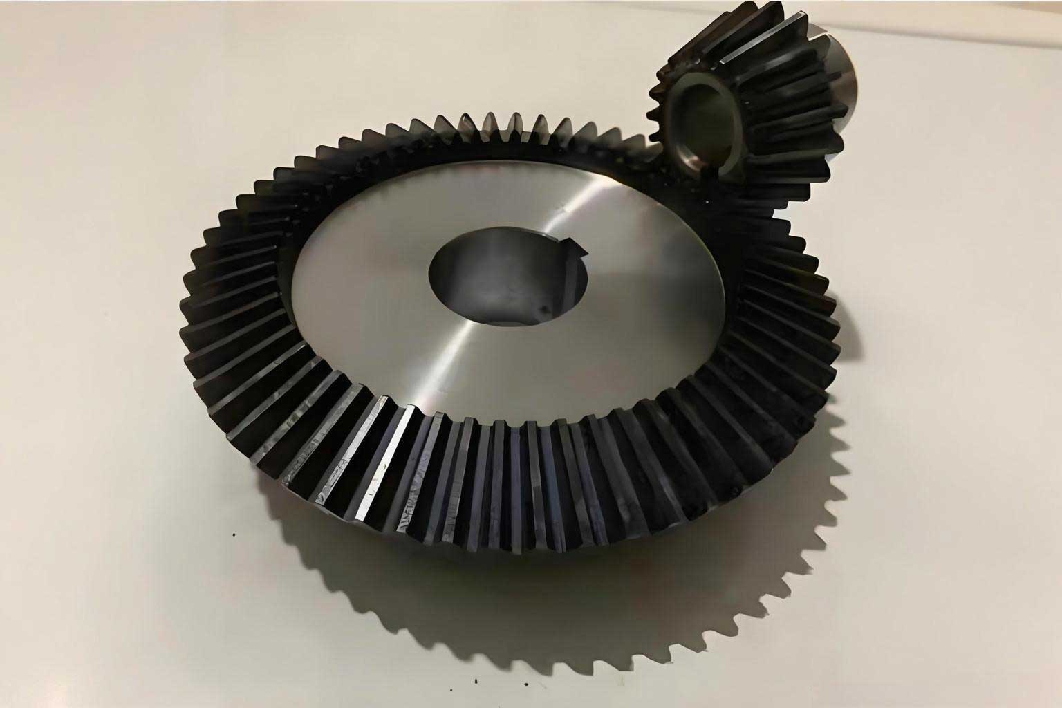
My research shows that crack-pitting coupling significantly reduces the mesh stiffness of miter gears, and the dynamic response exhibits impact behavior that varies with the meshing period. As the coupling severity increases, the impact becomes more severe, and sidebands appear near the meshing frequency harmonics in the frequency domain. I verified these findings through both finite element analysis and vibration tests. The experimental data and theoretical results show the same trend, with errors between 2% and 8%. This confirms the correctness of my proposed method and provides a theoretical basis for fault diagnosis and maintenance of miter gear transmission systems.
To calculate the time-varying mesh stiffness of healthy miter gears, I use the potential energy method and treat each tooth as a variable cross-section cantilever beam. I slice the miter gear tooth along the face width direction into several thin slices, and each slice is approximated as a spur gear slice. The mesh stiffness of each slice is obtained by integrating the deformation energy. The total mesh stiffness is the sum of all slices. I consider five stiffness components: bending stiffness \(k_b\), shear stiffness \(k_s\), axial compression stiffness \(k_a\), Hertzian contact stiffness \(k_h\), and fillet foundation stiffness \(k_f\). For a single slice \(i\), the mesh stiffness is:
$$ k_{mi} = \frac{1}{\frac{1}{k_h} + \frac{1}{k_{b1}} + \frac{1}{k_{s1}} + \frac{1}{k_{a1}} + \frac{1}{k_{f1}} + \frac{1}{k_{b2}} + \frac{1}{k_{s2}} + \frac{1}{k_{a2}} + \frac{1}{k_{f2}}} $$
where subscripts 1 and 2 denote the driving and driven gear slices, respectively. The total mesh stiffness is:
$$ k_m = \sum_{i=1}^{j} k_{mi} $$
where \(j\) is the number of slices. The energy stored in the gear tooth includes Hertzian contact energy \(U_h\), fillet foundation energy \(U_f\), axial compression energy \(U_a\), shear energy \(U_s\), and bending energy \(U_b\). These energies are related to the forces and stiffnesses as follows:
$$ U_h = \frac{F^2}{2k_h}, \quad U_f = \frac{F^2}{2k_f}, \quad U_a = \frac{F^2}{2k_a}, \quad U_s = \frac{F^2}{2k_s}, \quad U_b = \frac{F^2}{2k_b} $$
For a miter gear, the contact line length varies with time due to the helix angle. I model the contact line length as a piecewise function. When the transverse contact ratio \(\varepsilon_\alpha\) is greater than the overlap contact ratio \(\varepsilon_\beta\), the contact line length \(l(t)\) for one tooth pair is:
$$ l(t) = \begin{cases}
\frac{p_{bt}}{\sin \beta_b} \cdot \frac{t}{T_m}, & 0 < t < \varepsilon_\beta T_m \\
\frac{p_{bt}}{\sin \beta_b}, & \varepsilon_\beta T_m < t < \varepsilon_\alpha T_m \\
\frac{p_{bt}}{\sin \beta_b} \left( \frac{T_m + \varepsilon_\gamma T_m – t}{T_m} \right), & \varepsilon_\alpha T_m < t < \varepsilon_\gamma T_m \\
0, & \varepsilon_\gamma T_m < t < (M+1)T_m
\end{cases} $$
where \(p_{bt}\) is the base pitch, \(\beta_b\) is the base helix angle, \(T_m\) is the meshing period, \(\varepsilon_\gamma\) is the total contact ratio, and \(M\) is the largest integer less than \(\varepsilon_\gamma\). The total contact line for multiple teeth in mesh is obtained by summing the individual contact lines.
I use an improved method to calculate the bending, shear, and axial compression stiffness. The tooth is treated as a cantilever beam attached to the root circle. When the base circle radius is larger than the root circle radius, the integration is performed from the root circle to the engagement point. When the base circle radius is smaller than the root circle radius, the integration includes the portion between the base circle and the root circle. The bending stiffness \(k_b\), shear stiffness \(k_s\), and axial compression stiffness \(k_a\) are derived as:
$$ \begin{aligned}
k_b &= \int_{0}^{d} \frac{1}{E \left[ \frac{3(1+\cos\alpha_1)\sin\alpha_1 – 3\cos\alpha_1 \cos\alpha \cos\alpha_1}{2L} \right]^2 \frac{dy}{I_x}} \\
k_s &= \int_{0}^{d} \frac{1.2(1+\nu)\cos^2\alpha_1}{GA_x} dy \\
k_a &= \int_{0}^{d} \frac{\sin^2\alpha_1}{EA_x} dy
\end{aligned} $$
where \(E\) is Young’s modulus, \(G\) is the shear modulus, \(\nu\) is Poisson’s ratio, \(L\) is the tooth length, \(d\) is the distance from the engagement point to the root, \(A_x\) is the cross-sectional area, and \(I_x\) is the area moment of inertia. The detailed expressions depend on whether the base circle radius is larger or smaller than the root circle radius. I also include the fillet foundation stiffness \(k_f\), which is split into radial and axial components. The radial foundation stiffness \(k_{tf}\) and axial foundation stiffness \(k_{af}\) are:
$$ k_{tf} = \frac{1}{\frac{\cos^2\alpha}{E} \left( L^* \left( \frac{u_f}{S_f} \right)^2 + M^* \frac{u_f}{S_f} + P^* (1 + Q^* \tan^2\alpha) \right)} $$
$$ k_{af} = \frac{1}{\int_{0}^{R_r} \frac{(x \sin\alpha – x_1 \sin\alpha_1)^2}{E I_{af}(x_1)} dx_1} $$
where \(L^*, M^*, P^*, Q^*, u_f, S_f\) are geometric parameters, \(R_r\) is the root circle radius, and \(I_{af}\) is the moment of inertia of the fillet foundation. The total foundation stiffness \(k_f\) is:
$$ k_f = \frac{k_{tf} k_{af}}{k_{tf} + k_{af}} $$
For the Hertzian contact stiffness, I use an improved formula that accounts for the contact line length \(l\) and the load \(F\):
$$ k_h = \frac{2 E^{0.9} l^{0.8} F^{0.1}}{1.275} $$
where \(E^* = 1/(\frac{1-\nu_1^2}{E_1} + \frac{1-\nu_2^2}{E_2})\). This formula captures the nonlinear relationship between contact stiffness and load. I also consider the effect of the relief groove, which is often machined on miter gears to allow tool exit. The relief groove width \(L_t\) affects the foundation stiffness. As \(L_t\) increases, the mesh stiffness of the miter gear pair increases slightly, but the fluctuation remains almost unchanged. I calculated the mesh stiffness for different relief groove widths, and the results are summarized in Table 1.
| Relief groove width \(L_t\) (mm) | Average mesh stiffness (\(\times 10^9\) N/m) | Stiffness fluctuation (%) |
|---|---|---|
| 0 | 2.85 | 14.2 |
| 5 | 2.92 | 14.0 |
| 10 | 2.98 | 13.8 |
| 15 | 3.05 | 13.6 |
Next, I model the pitting fault. Pitting occurs on the tooth surface and is often idealized as a cylindrical pit. I define the pit by its center distance \(y_{sp}\) from the end face, the pit depth \(d_{sp}\), and the pit radius \(R_{sp}\). The pit reduces the effective contact line length and the cross-sectional area of the tooth. I derive the reduced area \(A’_x\) and reduced moment of inertia \(I’_x\) as:
$$ A’_x = (h_x + h’_x) L_x $$
$$ I’_x = \frac{1}{12} (h_x + h’_x)^3 dy $$
where \(h_x\) is the half tooth thickness at position \(x\), and \(h’_x\) is the additional thickness change due to pitting. The pitting reduces the Hertzian contact stiffness and the bending, shear, and axial compression stiffness. I consider four pitting levels: slight, transitional, moderate, and severe. The number of pits and their radii are increased to represent these levels. Table 2 shows the pitting parameters.
| Pitting level | Number of pits | Pit radius (mm) | Pit depth (mm) |
|---|---|---|---|
| Slight | 3 | 0.3 | 0.3 |
| Transitional | 6 | 0.3 | 0.3 |
| Moderate | 6 | 0.4 | 0.3 |
| Severe | 12 | 0.4 | 0.3 |
For crack modeling, I assume a straight crack at the tooth root. The crack depth \(q_i\) is defined as a percentage of the maximum distance \(q_{max}\) from the crack location to the tooth centerline. I use four crack levels: 10%, 30%, 50%, and 70%. The crack reduces the effective cross-sectional area and the area moment of inertia, which affects the bending and shear stiffness. The axial compression stiffness and Hertzian stiffness are mainly affected by pitting. When a crack and pitting coexist, the effective area and moment of inertia are determined by the dominant damage. I derive the coupled stiffness for four cases: (1) crack does not affect pitting, (2) crack begins to affect pitting, (3) crack dominates, and (4) crack affects the entire tooth surface. The coupled bending stiffness \(k_{bc}\) and shear stiffness \(k_{sc}\) are obtained by integrating the reduced section properties. For example, in the case where the crack dominates, the cross-sectional area and moment of inertia are:
$$ A_x = (h_a + h_x) L_x $$
$$ I_x = \frac{1}{12} (h_a + h_x)^3 L_x $$
where \(h_a\) is the distance from the crack tip to the tooth centerline. The detailed expressions for all four cases are lengthy, but they follow the same integration principle. I calculated the time-varying mesh stiffness for different crack-pitting coupling levels. Table 3 shows the stiffness reduction percentages at two representative time instants \(t_1\) and \(t_2\), where \(t_1\) is when the tooth engages the first row of pits, and \(t_2\) is when it engages the second row.
| Coupling case | Pitting reduction (%) | Crack reduction (%) | Total coupling reduction (%) | Pitting influence ratio (%) | Crack influence ratio (%) |
|---|---|---|---|---|---|
| Slight crack + slight pitting | 1.66 | 0.35 | 2.01 | 82.59 | 17.41 |
| Transitional crack + slight pitting | 1.66 | 1.34 | 2.89 | 57.44 | 46.37 |
| Moderate crack + slight pitting | 1.66 | 3.05 | 4.66 | 35.62 | 65.45 |
| Severe crack + slight pitting | 1.66 | 6.76 | 7.92 | 20.96 | 85.35 |
| Slight crack + transitional pitting | 3.60 | 0.35 | 3.95 | 91.14 | 8.86 |
| Transitional crack + transitional pitting | 3.60 | 1.34 | 4.85 | 74.27 | 27.63 |
| Moderate crack + transitional pitting | 3.60 | 3.05 | 5.79 | 62.18 | 52.68 |
| Severe crack + transitional pitting | 3.60 | 6.76 | 9.29 | 38.75 | 72.7 |
| Slight crack + moderate pitting | 5.11 | 0.35 | 5.46 | 93.59 | 6.41 |
| Transitional crack + moderate pitting | 5.11 | 1.34 | 6.08 | 84.05 | 22.04 |
| Moderate crack + moderate pitting | 5.11 | 3.05 | 6.98 | 73.21 | 43.70 |
| Severe crack + moderate pitting | 5.11 | 6.76 | 10.40 | 49.13 | 65.00 |
| Slight crack + severe pitting | 5.10 | 0.98 | 6.08 | 83.88 | 16.12 |
| Transitional crack + severe pitting | 5.10 | 4.46 | 9.05 | 56.35 | 49.28 |
| Moderate crack + severe pitting | 5.10 | 6.76 | 10.40 | 49.04 | 65.00 |
| Severe crack + severe pitting | 5.10 | 14.5 | 17.60 | 28.98 | 82.39 |
I also compared my analytical results with finite element results. I established a three-dimensional finite element model of a miter gear pair in ANSYS. The pinion was given a speed of 10 rad/s and the gear was loaded with a torque of 200 N·m. The contact was set as frictional. The mesh was refined around the pits. The simulation results showed that the stress and strain were concentrated on the meshing surface. I compared the mesh stiffness obtained from the potential energy method and the finite element method for healthy and faulty gears. The maximum error was less than 2.5%. This confirms the accuracy of my analytical model. Table 4 shows the comparison for one representative case.
| Method | Average mesh stiffness (\(\times 10^9\) N/m) | Minimum mesh stiffness (\(\times 10^9\) N/m) | Error (%) |
|---|---|---|---|
| Analytical | 2.98 | 2.54 | – |
| Finite element | 2.91 | 2.49 | 2.4 |
After obtaining the time-varying mesh stiffness with crack-pitting coupling, I established a 48-DOF dynamic model for the two-stage miter gear transmission system. The model includes bending, torsion, axial, and swing motions. I used the lumped parameter method. The model considers time-varying mesh stiffness, comprehensive transmission error, support stiffness, torsional stiffness, friction, and the relief groove. The differential equations of motion are derived using Newton’s second law. For the first-stage left driving gear, the equations are:
$$ \begin{aligned}
m_{AL}^1 \ddot{x}_{AL}^1 &+ k_{ALx}^1 f(x_{AL}^1) + k_{Atx}^1 (x_{AL}^1 – x_{AR}^1) + c_{ALx}^1 \dot{x}_{AL}^1 + c_{Atx}^1 (\dot{x}_{AL}^1 – \dot{x}_{AR}^1) \\
&= -k_{mL}^1 f(\delta_L^1) \cos\beta \sin\psi – c_{mL}^1 \dot{\delta}_L^1 \cos\beta \sin\psi + F_{fx}^{AL} \\
m_{AL}^1 \ddot{y}_{AL}^1 &+ k_{ALy}^1 f(y_{AL}^1) + k_{Aty}^1 (y_{AL}^1 – y_{AR}^1) + c_{ALy}^1 \dot{y}_{AL}^1 + c_{Aty}^1 (\dot{y}_{AL}^1 – \dot{y}_{AR}^1) \\
&= -k_{mL}^1 f(\delta_L^1) \cos\beta \cos\psi – c_{mL}^1 \dot{\delta}_L^1 \cos\beta \cos\psi + F_{fy}^{AL} \\
m_{AL}^1 \ddot{z}_{AL}^1 &+ k_{ALz}^1 f(z_{AL}^1) + k_{Atz}^1 (z_{AL}^1 – z_{AR}^1) + c_{ALz}^1 \dot{z}_{AL}^1 + c_{Atz}^1 (\dot{z}_{AL}^1 – \dot{z}_{AR}^1) \\
&= k_{mL}^1 f(\delta_L^1) \sin\beta + c_{mL}^1 \dot{\delta}_L^1 \sin\beta \\
I_{AL}^1 \ddot{\theta}_{xAL}^1 &+ k_{\theta xAL}^1 \dot{\theta}_{xAL}^1 + c_{\theta xAL}^1 \dot{\theta}_{xAL}^1 = -k_{mL}^1 f(\delta_L^1) \sin\beta \cos\psi R_{AL} + T_{AL} \\
I_{AL}^1 \ddot{\theta}_{yAL}^1 &+ k_{\theta yAL}^1 \dot{\theta}_{yAL}^1 + c_{\theta yAL}^1 \dot{\theta}_{yAL}^1 = -k_{mL}^1 f(\delta_L^1) \sin\beta \sin\psi R_{AL} + T_{AL}
\end{aligned} $$
Similar equations are written for all eight gears (two stages, each with left and right helical gears). The total number of degrees of freedom is 48. The internal excitation includes the time-varying mesh stiffness and the comprehensive transmission error. I represent these as Fourier series:
$$ k_m(t) = k_{AVG} \left[ 1 + \sum_{l=1}^{L} \varepsilon_l \cos(l \omega t + \phi_l) \right] $$
$$ e(t) = e_m + \sum_{l=1}^{L} e_l \sin(l \omega t + \phi_l) $$
where \(k_{AVG}\) is the average mesh stiffness, \(\varepsilon_l\) is the stiffness fluctuation coefficient, \(e_m\) is the mean error, \(e_l\) is the error fluctuation coefficient, and \(L\) is the expansion order. The mesh damping \(c_m\) and torsional damping \(c_t\) are calculated as:
$$ c_m = 2 \zeta \sqrt{k_{AVG} m_c} $$
where \(\zeta\) is the damping ratio and \(m_c\) is the equivalent mass. I also calculate the friction coefficient using an elastohydrodynamic lubrication (EHL) model. The friction coefficient \(\mu\) depends on the slide-to-roll ratio \(SR\), the maximum contact pressure \(P_h\), the dynamic viscosity \(v_0\), and the surface roughness \(S\). The formula is:
$$ \mu = e^{f(SR, P_h, v_0, S)} P_h^{c_2} |SR|^{c_3} v_e^{c_4} v_0^{c_5} R^{c_6} S^{c_7} $$
where \(f(SR, P_h, v_0, S)\) is a polynomial function, and \(c_1\) to \(c_9\) are empirical parameters. I used the values listed in Table 5.
| Parameter | \(c_1\) | \(c_2\) | \(c_3\) | \(c_4\) | \(c_5\) | \(c_6\) | \(c_7\) | \(c_8\) | \(c_9\) |
|---|---|---|---|---|---|---|---|---|---|
| Value | -8.92 | 1.05 | 1.05 | -0.34 | 2.82 | -0.11 | 0.74 | -0.37 | 0.64 |
I solved the 48-DOF differential equations using the Runge-Kutta method. The input speed was 1800 r/min and the input torque was 200 N·m. The gear parameters are listed in Table 6.
| Parameter | First stage driving | First stage driven | Second stage driving | Second stage driven |
|---|---|---|---|---|
| Number of teeth | 25 | 60 | 25 | 75 |
| Module (mm) | 2 | 2 | 2 | 2 |
| Helix angle (°) | 15 | 15 | 15 | 15 |
| Pressure angle (°) | 20 | 20 | 20 | 20 |
| Mass (kg) | 2 | 5 | 2 | 5 |
| Relief groove width (mm) | 3 | 3 | 3 | 3 |
| Relief groove radius (mm) | 26 | 58 | 26 | 72 |
| Total face width (mm) | 43 | 43 | 43 | 43 |
| Shaft hole radius (mm) | 20 | 20 | 20 | 20 |
| Poisson’s ratio | 0.3 | 0.3 | 0.3 | 0.3 |
| Moment of inertia (kg·m²) | 5 | 10 | 5 | 10 |
| Support stiffness (N/m) | 1×10⁹ | 1×10⁹ | 1×10⁹ | 1×10⁹ |
| Support damping (N·s/m) | 1×10⁵ | 1×10⁵ | 1×10⁵ | 1×10⁵ |
For healthy miter gears, the time-domain vibration signals are periodic and stable. The first-stage gear pair vibrates between -37.3 μm and -36.3 μm, and the second-stage gear pair vibrates between -67.6 μm and -65.1 μm. In the frequency domain, the main components are the meshing frequency \(f_m\), the second harmonic \(2f_m\), and the third harmonic \(3f_m\). No obvious sidebands are present. When crack-pitting coupling is introduced, the time-domain signal shows clear impacts. The amplitude of the impact region increases with the coupling severity. For the first-stage gear pair, the amplitude increases from 0.60 μm at 10% coupling to 1.16 μm at 70% coupling, which is a 132% increase compared to the healthy case. For the second-stage gear pair, the amplitude increases from 1.77 μm at 10% coupling to 6.02 μm at 70% coupling, which is a 381.6% increase. Table 7 summarizes the amplitude changes.
| Coupling level | First stage amplitude (μm) | Increase vs. healthy (%) | Second stage amplitude (μm) | Increase vs. healthy (%) |
|---|---|---|---|---|
| Healthy | 0.50 | 0 | 1.25 | 0 |
| 10% | 0.60 | 20 | 1.77 | 41.6 |
| 30% | 0.71 | 42 | 2.43 | 94.4 |
| 50% | 0.84 | 68 | 3.57 | 185.6 |
| 70% | 1.16 | 132 | 6.02 | 381.6 |
In the frequency domain, the crack-pitting coupling generates sidebands around the meshing frequency harmonics. For the first-stage gear pair, the sideband spacing \(\Delta f\) is 30 Hz, which corresponds to the rotation frequency of the cracked gear. For the second-stage gear pair, the sideband spacing is 12.5 Hz. As the coupling severity increases, the amplitude of the sidebands increases. This indicates that the system becomes less stable and the vibration level increases. The sidebands can be used to identify the presence and severity of crack-pitting coupling in miter gears.
I also compared the maximum vibration displacement in the y-direction for different coupling levels. The second-stage gear pair shows a much stronger response than the first-stage gear pair. For the same coupling level, the second-stage vibration displacement increases more rapidly. This suggests that the main vibration response of the two-stage miter gear transmission system is concentrated in the second stage. Table 8 shows the maximum displacement comparison.
| Coupling level | First stage max displacement (μm) | Second stage max displacement (μm) |
|---|---|---|
| Healthy | 0.52 | 1.28 |
| 10% | 0.62 | 1.80 |
| 30% | 0.73 | 2.48 |
| 50% | 0.86 | 3.62 |
| 70% | 1.18 | 6.10 |
To validate my theoretical model, I conducted vibration tests on a two-stage miter gear transmission system. I purchased wide helical gears and cut them into narrow helical gears using wire electrical discharge machining. Then I assembled left and right helical gears into miter gears using positioning pins. I machined cracks of different depths using wire cutting and fabricated pitting of different levels using electrical discharge machining. The test rig consisted of a control cabinet, an AC servo motor, a miter gearbox, accelerometers, a torque sensor, a magnetic powder brake, and a data acquisition system. The input speed was set to 1800 r/min and the torque to 200 N·m. I collected acceleration signals and integrated them twice to obtain displacement signals. The experimental results showed the same trend as the theoretical results. The error between theory and experiment was between 2% and 8%, which is acceptable given the simplifications in the theoretical model. Table 9 compares the theoretical and experimental maximum displacements for different coupling levels.
| Coupling level | Theoretical displacement (μm) | Experimental displacement (μm) | Error (%) |
|---|---|---|---|
| Healthy | 1.28 | 1.35 | 5.2 |
| 10% | 1.80 | 1.92 | 6.3 |
| 30% | 2.48 | 2.65 | 6.4 |
| 50% | 3.62 | 3.88 | 6.7 |
| 70% | 6.10 | 6.55 | 6.9 |
Based on my research, I draw the following conclusions. First, the relief groove width affects the mesh stiffness of miter gears. As the relief groove width increases, the mesh stiffness increases slightly, but the fluctuation remains almost unchanged. Second, crack-pitting coupling significantly reduces the mesh stiffness. In the early stage, pitting dominates and its influence ratio is between 82.59% and 93.59%. In the intermediate stage, both pitting and crack contribute, with pitting influence between 35.62% and 84.50% and crack influence between 22.04% and 65.45%. In the late stage, crack dominates, with crack influence between 65.00% and 85.35% and pitting influence between 20.96% and 49.13%. Third, the dynamic response of the two-stage miter gear transmission system shows impact behavior that varies with the meshing period. As the coupling severity increases, the impact becomes more severe. Fourth, the frequency response exhibits sidebands near the meshing frequency harmonics. The sideband amplitude increases with coupling severity, indicating reduced system stability. Fifth, the second-stage gear pair has a stronger vibration response than the first-stage gear pair, and the main vibration energy is concentrated in the second stage. Sixth, the experimental results agree well with the theoretical predictions, with errors between 2% and 8%. This validates the correctness of my proposed method and the 48-DOF dynamic model.
My work provides a new analytical method for calculating the time-varying mesh stiffness of miter gears with crack-pitting coupling. I have established a 48-DOF coupled dynamic model that includes bending, torsion, axial, and swing motions. I have also verified the model through finite element analysis and vibration experiments. The results can be used for fault diagnosis and condition monitoring of miter gear transmission systems. In future work, I plan to extend the model to include multiple faulty gears and different fault combinations. I will also consider nonlinear factors such as backlash and time-varying friction to further improve the accuracy of the dynamic model. This will help improve the safety and reliability of miter gear transmission systems in high-torque applications.