
In this article, I will explore a method for automatically measuring tooth pitch deviation in involute cylindrical spur gears using machine vision technology. The approach leverages an image measurement system to capture end-face images of spur gears and employs a series of image processing algorithms to compute deviations, including single pitch deviation, cumulative pitch deviation, and total cumulative pitch deviation. Machine vision offers advantages such as high precision, non-contact measurement, speed, and automation, making it suitable for industrial applications. I will detail the measurement principles, algorithm design, experimental setup, and results, emphasizing the use of formulas and tables for clarity. Throughout, the term ‘spur gears’ will be frequently referenced to highlight the focus on this common gear type.
The field of machine vision has evolved significantly since its inception in the 1950s, with applications spanning manufacturing, healthcare, and agriculture. For spur gears, traditional contact-based measurement tools like coordinate measuring machines or dedicated gauges are often slow, labor-intensive, and prone to inaccuracies. Thus, I propose an image-based method that can enhance efficiency and precision. The core idea involves capturing images of spur gears, processing them to extract geometric features, and calculating pitch deviations based on defined standards. This method aligns with trends toward smart manufacturing and automated quality control.
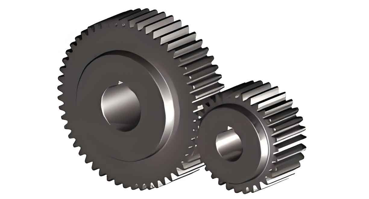
Before delving into details, I will insert a visual reference for spur gears to illustrate the subject matter. This image provides a clear view of a typical spur gear, which will aid in understanding the geometric parameters discussed later.
The measurement principle relies on image measurement fundamentals. An imaging system, comprising a camera and lens, projects the gear’s surface onto a photoelectric sensor, converting light into electronic images. These images are processed on a computer to extract features like gear contours and intersection points with reference circles. For instance, to measure the arc length between two points A and B on the pitch circle of spur gears, the pixel coordinates are used. Let the pixel coordinates of A be $$(u_a, v_a)$$ and B be $$(u_b, v_b)$$. The actual arc length AB is calculated using the pixel equivalent $$ \tau $$ (in mm/pixel), which represents the magnification of the imaging system:
$$ AB = \tau \sqrt{(u_a – u_b)^2 + (v_a – v_b)^2} $$
Here, $$ \tau $$ is determined through system calibration, often using a standard chessboard or scale. This formula underpins all geometric measurements for spur gears, as distances in pixel space are converted to real-world dimensions. The accuracy hinges on precise calibration, which I will address in the algorithm section.
Moving to algorithm design, the process involves multiple steps: image preprocessing, system calibration, gear contour and feature extraction, pitch circle construction, and pitch parameter calculation. Each step is critical for ensuring reliable measurements of spur gears. I will outline these with formulas and tables to summarize key aspects.
First, image preprocessing enhances image quality by reducing noise and highlighting gear contours. The flowchart includes Gaussian filtering, binarization, and edge detection. For spur gears, binarization thresholds are set based on pixel intensity differences between the background and gear edges. Edge detection uses the Sobel operator, which computes gradients to identify boundaries. The horizontal and vertical derivatives for a pixel $$ P_5 $$ are given by:
$$ P_{5x} = (P_3 – P_1) + 2 \cdot (P_6 – P_4) + (P_9 – P_7) $$
$$ P_{5y} = (P_7 – P_1) + 2 \cdot (P_8 – P_2) + (P_9 – P_3) $$
Where $$ P_1 $$ to $$ P_9 $$ represent neighboring pixels. This operator efficiently extracts edges, which are essential for subsequent contour analysis of spur gears.
Next, system calibration corrects lens distortions and determines the pixel equivalent. I adopt Zhang’s method for single-plane chessboard calibration. Distortions include radial and tangential components. For radial distortion, corrected coordinates $$(x_r, y_r)$$ are derived from uncorrected coordinates $$(x_p, y_p)$$:
$$ x_r = x_p (1 + k_1 r^2 + k_2 r^4 + k_3 r^6) $$
$$ y_r = y_p (1 + k_1 r^2 + k_2 r^4 + k_3 r^6) $$
Here, $$ r $$ is the distance from the optical center, and $$ k_1, k_2, k_3 $$ are radial distortion coefficients. For tangential distortion:
$$ x_r = x_p [1 + 2 p_1 r^2 + p_2 (r^2 + 2 x^2)] $$
$$ y_r = y_p [1 + p_1 (r^2 + 2 y^2) + 2 p_2 x] $$
Where $$ p_1, p_2 $$ are tangential distortion coefficients. The camera intrinsic matrix $$ M $$ provides the pixel equivalent:
$$ M = \begin{bmatrix} f_x & 0 & u_0 \\ 0 & f_y & v_0 \\ 0 & 0 & 1 \end{bmatrix} = \begin{bmatrix} f/d_x & 0 & u_0 \\ 0 & f/d_y & v_0 \\ 0 & 0 & 1 \end{bmatrix} $$
In this matrix, $$(u_0, v_0)$$ is the principal point, $$ d_x, d_y $$ are pixel dimensions, and $$ f $$ is focal length. The pixel equivalent $$ \tau $$ is obtained from $$ f_x $$ and $$ f_y $$, typically as the average of $$ 1/(f_x/f) $$ and $$ 1/(f_y/f) $$. Calibration ensures accurate scaling for measuring spur gears.
Gear contour and feature extraction involve isolating the gear’s outer and inner boundaries. After preprocessing, Sobel edge detection yields contour points. For spur gears, I fit circles to these contours using least squares to find the gear center $$(x_0, y_0)$$. The gear center is computed as the average of outer and inner fitted circle centers. Then, the addendum circle radius $$ r_a $$ and dedendum circle radius $$ r_f $$ are determined. The addendum radius is found by constructing a convex hull around the outer contour and averaging distances from the gear center to intersection points. The dedendum radius is derived from the minimum distance of outer contour points to the center, with points in a range $$[d_{\text{min}}, d_{\text{min}} + d] $$ considered. The number of teeth $$ z $$ is counted by intersecting a circle at the mean of $$ r_a $$ and $$ r_f $$ with the outer contour, yielding twice the tooth count. The module $$ m $$ is calculated from the addendum radius:
$$ m’ = \frac{2 r_a}{z + 2} $$
This value is compared to standard module series to select the closest standard $$ m $$. These parameters are fundamental for analyzing spur gears.
Pitch circle construction uses the module and tooth count. The pitch circle radius $$ r $$ for spur gears is:
$$ r = \frac{m z}{2} $$
With the gear center, a circle of radius $$ r $$ is drawn, intersecting the gear轮廓 to obtain points for pitch deviation calculation. The intersection points are sorted clockwise, and their angles $$ \theta_i $$ relative to the x-axis are computed.
Pitch parameter calculation follows definitions from gear standards. The theoretical pitch $$ p $$ for spur gears is:
$$ p = \pi m $$
The actual pitch for the i-th tooth, based on left or right flank, is:
$$ p_i = \frac{m z}{2} (\theta_{i+2} – \theta_i) \quad \text{or} \quad p_i = \frac{m z}{2} (\theta_{i+1} – \theta_{i-1}) $$
Angle differences are adjusted to be between 0 and $$ 2\pi $$. The i-th pitch deviation $$ f_{pi} $$ is:
$$ f_{pi} = p_i – p $$
Single pitch deviation $$ f_{pt} $$ is the maximum absolute value of $$ f_{pi} $$. For cumulative deviations, let k be an integer less than $$ z/8 $$ or $$ z/6 $$ as per standards. The k-tooth cumulative deviation $$ F_{pi} $$ is:
$$ F_{pi} = \max \sum_{j=i}^{i+k-1} f_{pj} $$
Total cumulative pitch deviation $$ F_p $$ is:
$$ F_p = \max(F_{pk}) – \min(F_{pk}) $$
Where $$ F_{pk} = \sum_{j=1}^{k} f_{pj} $$. These formulas enable comprehensive evaluation of spur gears’ pitch accuracy.
To summarize algorithm parameters, I present a table of key variables used in the measurement process for spur gears.
| Variable | Description | Typical Value/Range |
|---|---|---|
| $$ \tau $$ | Pixel equivalent (mm/pixel) | 0.00504 (from calibration) |
| $$ m $$ | Module (mm) | 0.6 (for tested spur gears) |
| $$ z $$ | Number of teeth | 14 (for tested spur gears) |
| $$ r_a $$ | Addendum circle radius (mm) | Derived from image |
| $$ r_f $$ | Dedendum circle radius (mm) | Derived from image |
| $$ k_1, k_2, k_3 $$ | Radial distortion coefficients | Calibration-dependent |
| $$ p_1, p_2 $$ | Tangential distortion coefficients | Calibration-dependent |
Now, I describe the experimental system and measurement results. The image measurement system includes a high-resolution industrial camera (e.g., CMOS sensor with 4320×2430 resolution), a fixed-focus lens (16 mm focal length), LED lighting, a stage, and a computer. The system captures images of spur gears and processes them using software developed with OpenCV and PyQt5 for a user-friendly interface. Calibration with a chessboard yields a pixel equivalent of 0.00504 mm/pixel, ensuring precise measurements.
In testing, multiple images of spur gears were taken from different orientations. Image processing steps, as outlined, produced gear contours and feature points. For example, the convex hull and intersection points with addendum and dedendum circles were identified. The tested spur gears had $$ z = 14 $$ and $$ m = 0.6 $$, giving a pitch radius of 4.2 mm. Measurements were repeated to assess repeatability.
I present a table of pitch deviation measurements for a sample spur gear, based on left and right flanks. The data illustrates variations across teeth.
| Tooth Index (i) | Pitch Deviation (Left Flank, μm) | Pitch Deviation (Right Flank, μm) |
|---|---|---|
| 1 | -0.131 | -2.787 |
| 2 | -7.395 | -0.111 |
| 3 | 0.411 | -1.295 |
| 4 | -22.115 | 5.829 |
| 5 | 21.317 | -10.414 |
| 6 | 5.620 | -29.053 |
| 7 | 10.261 | 39.830 |
| 8 | -3.565 | -2.425 |
| 9 | -7.979 | 4.367 |
| 10 | 2.071 | -10.471 |
| 11 | 3.391 | -16.315 |
| 12 | -35.055 | 11.500 |
| 13 | 23.137 | -14.961 |
| 14 | 10.032 | 26.304 |
The maximum single pitch deviations were 35.055 μm (left) and 39.830 μm (right), showing consistency between flanks. Cumulative deviations were plotted, and total cumulative pitch deviations were approximately 41.137 μm (left) and 41.771 μm (right), further validating the method for spur gears.
Repeatability analysis involved 10 measurements of the same spur gear. The standard deviation $$ s $$ was computed using Bessel’s formula:
$$ s = \sqrt{\frac{\sum_{i=1}^{n} (x_i – \bar{x})^2}{n-1}} $$
Where $$ n $$ is the sample count, $$ x_i $$ are measurements, and $$ \bar{x} $$ is the mean. Results for single pitch deviation, cumulative pitch deviation (with $$ k=2 $$), and total cumulative deviation are summarized below.
| Measurement Number | Single Pitch Deviation (μm) | Cumulative Pitch Deviation (μm) | Total Cumulative Deviation (μm) |
|---|---|---|---|
| 1 | -13.008 | -24.929 | 41.162 |
| 2 | -2.293 | -16.271 | 37.407 |
| 3 | -5.422 | -19.124 | 30.106 |
| 4 | -2.149 | -15.767 | 35.282 |
| 5 | -2.308 | -12.294 | 39.482 |
| 6 | -5.468 | -19.219 | 35.579 |
| 7 | -13.031 | -23.790 | 41.883 |
| 8 | -14.740 | -25.566 | 40.874 |
| 9 | -8.755 | -17.944 | 38.465 |
| 10 | -0.130 | -7.526 | 41.137 |
| Standard Deviation (μm) | 5.317 | 5.688 | 3.671 |
The standard deviations are below 6 μm, indicating good repeatability. To further validate, I tested three groups of spur gears (10 gears per group) with repeated measurements of total cumulative deviation. The maximum standard deviations across groups were 5.014 μm, 5.314 μm, and 5.302 μm, confirming that the system achieves effective detection for spur gears with precision better than 6 μm.
In conclusion, the machine vision-based method for measuring tooth pitch deviation in spur gears demonstrates high accuracy, automation, and non-contact benefits. By integrating image preprocessing, calibration, feature extraction, and pitch calculation, it overcomes limitations of traditional tools. The use of formulas for distortion correction and pitch evaluation, along with tables for data summary, enhances clarity. This approach is suitable for quality control in manufacturing, especially for spur gears used in various mechanical systems. Future work could explore real-time processing or integration with other gear parameters like profile deviation. Overall, the method offers a reliable solution for advancing gear measurement technology.
Throughout this discussion, I have emphasized the importance of spur gears in mechanical transmissions and how machine vision can optimize their inspection. The algorithms and systems described here can be adapted to other gear types, but the focus remains on spur gears due to their simplicity and widespread use. By leveraging computational techniques, we can ensure that spur gears meet stringent accuracy standards, contributing to improved performance and longevity in applications such as automotive, robotics, and industrial machinery.