
Spur gears are fundamental components in mechanical transmission systems, and their operational health is critical for the reliability of industrial machinery. Operating in harsh environments, spur gears are susceptible to various failures such as tooth breakage, pitting, wear, and root cracks. Statistics indicate that gear-related faults constitute a significant proportion, approximately 80%, of failures in transmission systems. Among these, root cracks are particularly insidious as they initiate due to cyclic bending stress and can propagate, leading to catastrophic tooth breakage and system shutdown. Therefore, effective methods for not only detecting the presence but also quantifying the severity of cracks in spur gears are of paramount importance for predictive maintenance and operational safety.
Much of the existing research focuses on the qualitative detection of crack existence in gears. Techniques such as spectral kurtosis, various time-frequency analyses (STFT, Wigner-Ville, CWT, DWT), Hilbert-Huang Transform (HHT), and combinations of higher-order cumulants with Empirical Mode Decomposition (EMD) have been explored to identify the faint signatures of incipient damage. However, accurately determining the degree or severity of a crack—quantifying how far it has propagated—remains a challenging and crucial step towards precise residual life estimation and condition-based maintenance scheduling for spur gear systems. This gap motivates our research into a robust quantitative damage assessment methodology.
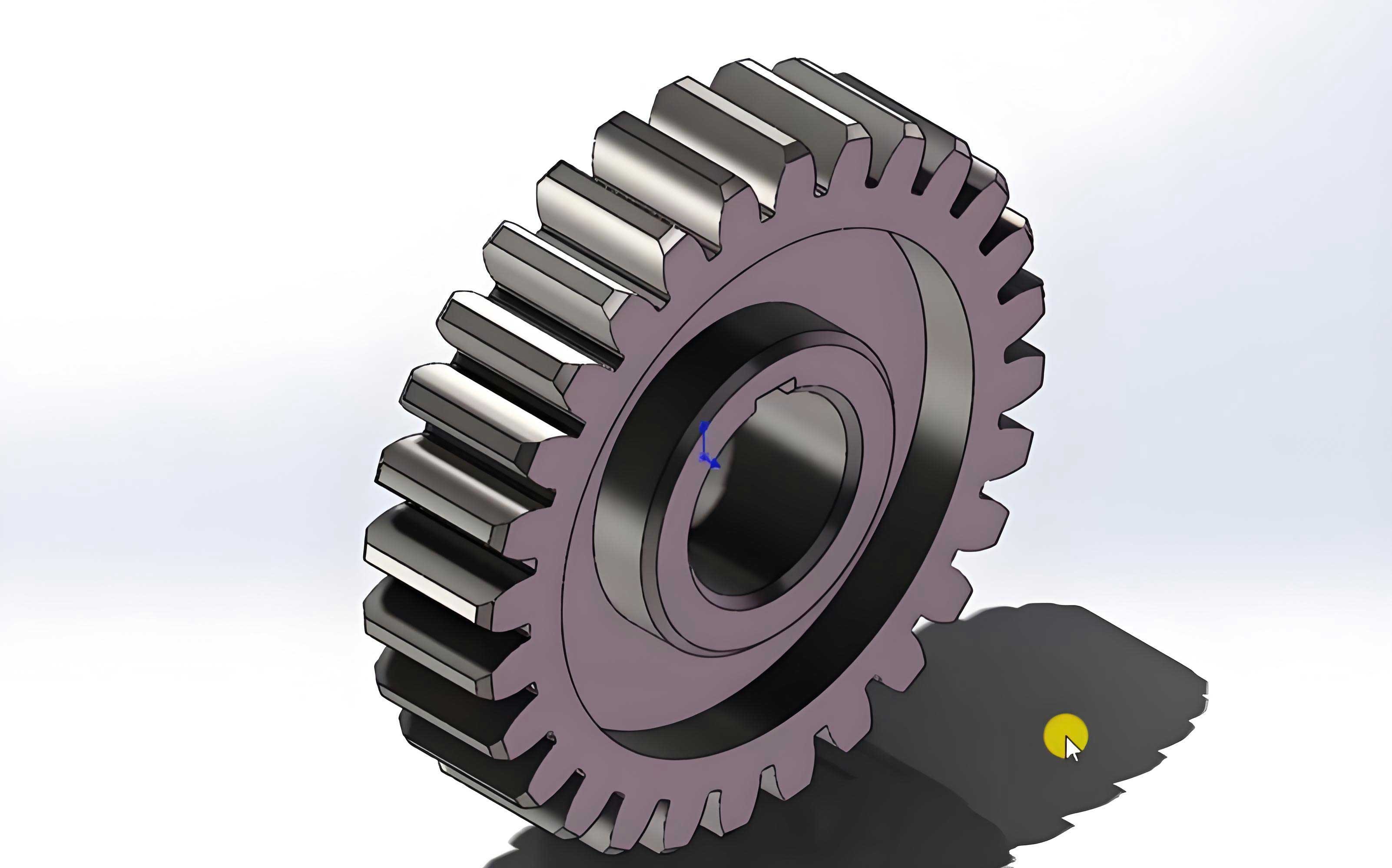
In this work, we propose an integrated approach combining Principal Component Analysis (PCA) and Grey Relational Analysis (GRA) to achieve degree-level detection of tooth root cracks in spur gear trains. Our methodology begins with establishing a detailed nonlinear dynamic model of a spur gear system that incorporates time-varying mesh stiffness altered by propagating root cracks. Simulation signals under different crack severity levels are generated from this model. Subsequently, a comprehensive set of fault-sensitive features is extracted from these signals using both time-domain and frequency-domain modern signal processing techniques. The core of our method lies in processing these multi-dimensional features: PCA is employed to optimize and reduce the dimensionality of the feature space, effectively distilling the most informative components. Then, GRA is used to compute relational degrees between the feature vector of an unknown state and pre-established standard pattern vectors representing defined damage levels. The damage degree is identified by the pattern yielding the maximum relational degree. Analysis based on simulation data demonstrates that our integrated PCA-GRA method offers a significant improvement in discrimination accuracy compared to direct thresholding on raw features, validating its effectiveness for quantitative fault diagnosis in spur gears.
Theoretical Foundation: Modeling Spur Gear Dynamics with Cracks
Dynamic Modeling of a Spur Gear Train
To accurately simulate the vibration response of faulty spur gears, we establish a lumped-parameter dynamic model. The model represents a single-stage spur gear transmission system, incorporating the driving motor and the load, resulting in a 6-degree-of-freedom (DOF) system. We assume ideal manufacturing, assembly, and lubrication conditions. Each spur gear has three potential DOFs (one rotational and two translational), while the motor and load have one rotational DOF each. Considering the internal excitation primarily from time-varying mesh stiffness and damping while neglecting friction, the vibration along the line-of-action (y-direction) is most critical; vibration in the x-direction (off line-of-action) is considered as damped free decay and is thus neglected for steady-state analysis. The schematic of the 6-DOF model is as follows.
The governing equations of motion for the spur gear system are:
$$
\begin{aligned}
m_1 \ddot{y}_1 &= F_k + F_c – F_u – F_{uc} \\
m_2 \ddot{y}_2 &= F_k + F_c – F_l – F_{lc} \\
I_1 \ddot{\theta}_1 &= M_{Pk} + M_{Pc} – R_{b1}(F_k + F_c) \\
I_2 \ddot{\theta}_2 &= R_{b2}(F_k + F_c) – M_{gk} – M_{gc} \\
I_m \ddot{\theta}_m &= M_1 – M_{Pk} – M_{pc} \\
I_b \ddot{\theta}_b &= -M_2 + M_{gk} + M_{gc}
\end{aligned}
$$
where the mesh force \(F_k\) and damping force \(F_c\) are defined as:
$$
\begin{aligned}
F_k &= k_t(t) (R_{b1}\theta_1 – R_{b2}\theta_2 – y_1 + y_2) \\
F_c &= c_t (\dot{R}_{b1}\theta_1 – \dot{R}_{b2}\theta_2 – \dot{y}_1 + \dot{y}_2)
\end{aligned}
$$
The bearing forces and motor/load coupling torques are given by:
$$
\begin{aligned}
F_u = k_1 y_1, &\quad F_{uc} = c_1 \dot{y}_1 \\
F_l = k_2 y_2, &\quad F_{lc} = c_2 \dot{y}_2 \\
M_{Pk} = k_p (\theta_m – \theta_1), &\quad M_{Pc} = c_p (\dot{\theta}_m – \dot{\theta}_1) \\
M_{gk} = k_g (\theta_2 – \theta_b), &\quad M_{gc} = c_g (\dot{\theta}_2 – \dot{\theta}_b)
\end{aligned}
$$
Here, \(k_t(t)\) is the crucial time-varying mesh stiffness of the spur gear pair, which is the primary carrier of fault information for a cracked tooth.
Modeling Tooth Root Crack and Time-Varying Mesh Stiffness
The presence of a root crack in a spur gear tooth significantly alters its flexibility, thereby modifying the overall mesh stiffness \(k_t(t)\). We model the crack as a straight line originating at the root fillet, propagating at an angle \(\nu\) relative to the tooth centerline, with a length \(q\). The calculation of mesh stiffness is based on the potential energy method.
For a healthy spur gear pair, the total potential energy in meshing includes Hertzian contact energy \(U_h\), bending energy \(U_b\), shear energy \(U_s\), axial compressive energy \(U_a\), and later, the fillet foundation energy \(U_f\). The corresponding stiffness components (\(k_h, k_b, k_s, k_a, k_f\)) are connected in series. The bending and shear energies for a single tooth are calculated by integrating along the tooth from the base circle to the load point:
$$
\begin{aligned}
U_h &= \frac{F^2}{2k_h} \\
U_b &= \frac{F^2}{2k_b} = \int_0^d \frac{[F_b(d-x) – F_a h]^2}{2EI_x} dx \\
U_s &= \frac{F^2}{2k_s} = \int_0^d \frac{1.2F_b^2}{2GA_x} dx \\
U_a &= \frac{F^2}{2k_a} = \int_0^d \frac{F_a^2}{2EA_x} dx
\end{aligned}
$$
where \(F\) is the total meshing force, decomposable into tangential (\(F_b\)) and radial (\(F_a\)) components. \(I_x\) and \(A_x\) are the area moment of inertia and cross-sectional area at a distance \(x\) from the base, respectively. For a healthy, symmetric spur gear tooth, \(I_x = \frac{1}{12}(2h_x)^3 L\) and \(A_x = 2h_x L\), where \(h_x\) is half the tooth thickness at section \(x\).
The fillet foundation stiffness \(k_f\) accounts for deformation of the gear body and is given by:
$$
\frac{1}{k_f} = \frac{\cos^2 \alpha}{EL} \left\{ L^*\left(\frac{\mu_f}{S_f}\right)^2 + M^*\left(\frac{\mu_f}{S_f}\right) + P^*(1 + Q^*\tan^2 \alpha) \right\}
$$
The coefficients \(L^*, M^*, P^*, Q^*\) are calculated using polynomial functions of parameters \(\theta_f\) and \(h_{fi} = r_f / r_{int}\):
$$
X_i^* = \frac{A_i}{\theta_f^2} + B_i h_{fi} + \frac{C_i h_{fi}}{\theta_f^2} + \frac{D_i}{\theta_f} + E_i h_{fi} + F_i
$$
The values for the constants \(A_i, B_i, …, F_i\) for each coefficient are summarized in the table below.
| Coefficient | \(A_i \times 10^{-5}\) | \(B_i \times 10^{-3}\) | \(C_i \times 10^{-4}\) | \(D_i \times 10^{-3}\) | \(E_i\) | \(F_i\) |
|---|---|---|---|---|---|---|
| \(L^*\) | -5.5740 | -1.9986 | -2.3015 | 4.7702 | 0.0271 | 6.8045 |
| \(M^*\) | 60.1110 | 28.1000 | -83.4310 | -9.9260 | 0.1624 | 0.9086 |
| \(P^*\) | -50.9520 | 185.5000 | 0.0538 | 53.3000 | 0.2895 | 0.9236 |
| \(Q^*\) | -6.2042 | 9.0889 | -4.0964 | 7.8297 | -0.1472 | 0.6904 |
For a spur gear pair in double-tooth engagement, the total effective mesh stiffness is the sum of the stiffnesses for the two engaged tooth pairs:
$$
k_t(t) = \sum_{i=1}^{2} \left( \frac{1}{\frac{1}{k_{h_i}} + \frac{1}{k_{b1,i}} + \frac{1}{k_{s1,i}} + \frac{1}{k_{a1,i}} + \frac{1}{k_{f1,i}} + \frac{1}{k_{b2,i}} + \frac{1}{k_{s2,i}} + \frac{1}{k_{a2,i}} + \frac{1}{k_{f2,i}}} \right)
$$
Effect of a Root Crack: A crack in the spur gear tooth root affects the bending and shear stiffness by changing the cross-sectional geometry. The Hertzian contact stiffness and axial compressive stiffness are assumed unchanged. For a section at distance \(x\) from the base, if the crack tip has not passed this section (\(x \leq g_c\)), the area moment of inertia and area become:
$$
I_x = \frac{1}{12}(h_{c1} + h_x)^3 L, \quad A_x = (h_{c1} + h_x)L
$$
For sections beyond the crack tip (\(x > g_c\)), the formulas revert to those of a healthy tooth. Here, \(h_{c1}\) is the distance from the crack root to the tooth centerline, and \(g_c\) is the horizontal distance from the root where \(h_x = h_{c1}\). Substituting these modified expressions for \(I_x\) and \(A_x\) into the energy equations allows for the calculation of the bending and shear stiffnesses of the cracked spur gear tooth, ultimately leading to the fault-modulated time-varying mesh stiffness \(k_t(t, q)\), which is a function of both time and crack depth \(q\).
The Proposed PCA-Grey Theory Methodology for Spur Gear Crack Severity Assessment
Feature Extraction and Dimensionality Reduction via PCA
From the simulated vibration signals (specifically the y-direction displacement or acceleration) of the spur gear system under various crack states, we extract a comprehensive set of \(n\) fault-sensitive features. For spur gear damage detection, we select six commonly used and effective statistical indicators:
- Kurtosis (Kur): Measures the “tailedness” of the signal distribution, sensitive to impulsive faults.
- Fourth-Order Moment (FM4): A normalized fourth-order moment, robust to speed and load variations.
- Spectrum Kurtosis (KS): The kurtosis computed in the frequency domain, indicating impulsiveness in specific frequency bands.
- Root Mean Square (RMS): Measures the overall energy level of the vibration signal.
- Mean Value: The average value of the signal.
- Statistical Parameter \(s_\alpha\): A relatively new indicator designed to be less sensitive to spurious vibrations compared to kurtosis, defined as:
$$ s_\alpha = \frac{ \frac{1}{N} \sum_{n=1}^{N} |x(n)-\bar{x}|^3 }{ \left( \frac{1}{N} \sum_{n=1}^{N} (x(n)-\bar{x})^2 \right)^{3/2} } $$
For \(m\) different pre-defined damage states (e.g., crack lengths from 0 to 1.5 mm in 0.1 mm increments), we construct an initial feature matrix \(\mathbf{X}\) of size \(m \times n\). Principal Component Analysis (PCA) is a statistical procedure that uses an orthogonal transformation to convert a set of possibly correlated variables (our \(n\) features) into a set of linearly uncorrelated variables called principal components (PCs). This transformation is defined in such a way that the first principal component accounts for the largest possible variance in the data, and each succeeding component accounts for the highest variance under the constraint of being orthogonal to the preceding ones.
Let the original feature vector be \(\mathbf{X} = [x_1, x_2, …, x_n]\). After PCA, we obtain a transformed vector \(\mathbf{Y} = [y_1, y_2, …, y_n]\), where the components \(y_i\) are uncorrelated. The contribution rate \(t_i\) of the \(i\)-th principal component \(y_i\) and the cumulative contribution rate \(t_{tm}\) of the first \(m\) PCs are calculated as:
$$
t_i = \frac{\lambda_i}{\sum_{k=1}^{n} \lambda_k}, \quad t_{tm} = \frac{\sum_{i=1}^{m} \lambda_i}{\sum_{k=1}^{n} \lambda_k}
$$
where \(\lambda_i\) is the eigenvalue (variance) corresponding to \(y_i\). We select the first \(p\) principal components such that their cumulative contribution rate \(t_{tp} > 95\%\). This reduced-dimension feature vector \(\mathbf{Y}_{reduced} = [y_1, y_2, …, y_p]\), where \(p < n\), retains most of the essential information from the original features while eliminating redundancy and noise, providing an optimized input for the subsequent pattern recognition stage in our spur gear diagnosis.
Damage Degree Identification Using Grey Relational Analysis
Grey Relational Analysis (GRA) is a method to measure the degree of similarity between sequences based on the geometric proximity of their development trends. In the context of spur gear fault diagnosis, we use it to quantify the closeness between the feature vector of an unknown state and the standard pattern vectors representing known damage degrees.
Let the feature sequence of the state under inspection be \(\mathbf{X}_0 = \{x_0(j)\}, j=1,2,…,p\). Let the standard pattern sequences for \(m\) pre-defined damage states be \(\mathbf{X}_i = \{x_i(j)\}, i=1,2,…,m, j=1,2,…,p\). The relational coefficient \(\gamma(x_0(j), x_i(j))\) between \(\mathbf{X}_0\) and \(\mathbf{X}_i\) at the \(j\)-th index is calculated as:
$$
\gamma(x_0(j), x_i(j)) = \frac{ \min_i \min_j |x_0(j)-x_i(j)| + \rho \, \max_i \max_j |x_0(j)-x_i(j)| }{ |x_0(j)-x_i(j)| + \rho \, \max_i \max_j |x_0(j)-x_i(j)| }
$$
where \(\rho\) is the distinguishing coefficient, typically set to 0.5. The overall grey relational degree \(\gamma_i\) between the unknown state and the \(i\)-th standard state is the average of the relational coefficients across all features:
$$
\gamma_i = \frac{1}{p} \sum_{j=1}^{p} \gamma(x_0(j), x_i(j))
$$
The damage degree of the unknown spur gear is then identified as corresponding to the standard state \(i^*\) that yields the maximum relational degree: \(i^* = \arg\max_i (\gamma_i)\). The value of \(\gamma_{i^*}\) itself can also be interpreted as a confidence measure for the diagnosis.
Integrated Damage Degree Detection Procedure
The complete flowchart for the spur gear crack damage degree detection, integrating PCA and GRA, is as follows:
- Modeling & Simulation: Establish the nonlinear dynamic model of the spur gear system. Calculate the time-varying mesh stiffness \(k_t(t, q)\) for different crack depths \(q\). Generate vibration signals for \(m\) damage states via numerical integration (e.g., 4th-order Runge-Kutta).
- Feature Extraction: For each damage state signal, compute the \(n\) pre-selected fault features (Kur, FM4, KS, RMS, Mean, \(s_\alpha\)).
- Standard Pattern & Test Vector Formation: Arrange the features from the \(m\) standard states into an \(m \times n\) matrix. For an unknown/test state (e.g., crack length = 1.05 mm), compute its feature vector and append it as the \((m+1)\)-th row.
- PCA Processing: Apply PCA to the entire \((m+1) \times n\) feature matrix. Select the first \(p\) principal components ensuring >95% cumulative variance. Obtain the reduced-dimension standard pattern matrix \(\mathbf{Y}_{std}\) (size \(m \times p\)) and the test vector \(\mathbf{Y}_{test}\) (size \(1 \times p\)).
- Grey Relational Analysis: Normalize \(\mathbf{Y}_{std}\) and \(\mathbf{Y}_{test}\). Calculate the grey relational degree \(\gamma_i\) between \(\mathbf{Y}_{test}\) and each row of \(\mathbf{Y}_{std}\).
- Damage Degree Determination: The damage degree of the test spur gear is assigned to the standard state \(i^*\) with \(\max(\gamma_i)\). The associated crack severity (e.g., crack length range) is reported.
Simulation Analysis and Validation for Spur Gears
We conduct a simulation study to validate the proposed method for detecting crack depths ranging from 0 mm to 1.5 mm in a spur gear pinion. The crack length is increased in steps of 0.1 mm, resulting in 16 distinct damage states (0.0, 0.1, …, 1.5 mm). The parameters for the spur gear pair and the system are listed in the tables below.
| Gear | Number of Teeth | Module (mm) | Pressure Angle (°) | Young’s Modulus (N/mm²) | Poisson’s Ratio | Face Width (mm) |
|---|---|---|---|---|---|---|
| Pinion | 19 | 2 | 20 | 2×10⁵ | 0.3 | 16 |
| Gear | 48 | 2 | 20 | 2×10⁵ | 0.3 | 16 |
| Parameter Name | Value |
|---|---|
| Pinion Mass (kg) | 0.96 |
| Gear Mass (kg) | 2.88 |
| Motor Inertia (kg·m²) | 0.0021 |
| Load Inertia (kg·m²) | 0.0105 |
| Mesh Frequency (Hz) | 570 |
| Motor Torque (N·m) | 11.9 |
| Load Torque (N·m) | 48.8 |
The time-varying mesh stiffness is computed for different crack depths (e.g., q=0, 0.5, 1.0, 1.5 mm) and incorporated into the dynamic model. The system’s dynamic response is solved numerically. Analysis of the time-domain signals reveals periodic impact signatures when the cracked spur gear tooth enters the mesh. Frequency-domain analysis shows significant sidebands around the mesh frequency harmonics (2X, 3X, etc.), with their amplitudes increasing as the crack propagates, confirming the modulation effect caused by the fault in the spur gear.
For the 16 standard states and one test state (crack length = 1.05 mm), we extract the 6 features, forming a 17×6 matrix. Applying PCA, we reduce the dimension to a smaller set of principal components. Using GRA on the PCA-processed data, we compute the grey relational degree between the test state and each standard state. The results show a clear peak in relational degree at the standard state corresponding to a 1.0 mm crack length, accurately indicating that the test spur gear’s damage lies within the 0.9-1.1 mm range. The maximum relational degree value obtained is 0.9972.
To highlight the advantage of our integrated method, we perform a comparison. When the grey relational analysis is applied directly to the original 6 features without PCA preprocessing, the resulting maximum relational degree is only 0.8585. This demonstrates that our PCA-GRA method achieves a **16% improvement** in the discrimination metric (relational degree value). Furthermore, the curve of relational degree versus damage level using the PCA-processed features shows a more monotonic and pronounced trend compared to the curve from raw features, leading to a more reliable and interpretable diagnosis for the condition of the spur gears.
Conclusion
This paper presented an integrated methodology combining Principal Component Analysis (PCA) and Grey Relational Theory (GRT) for the quantitative assessment of tooth root crack damage in spur gear systems. The approach begins with a physics-based nonlinear dynamic model of a spur gear train, which accurately simulates the vibration response under varying levels of crack severity. A suite of sensitive fault features is extracted from these signals. The core innovation lies in the two-stage processing of these features: PCA effectively compresses the multi-dimensional feature space, eliminating redundancy and noise to yield an optimized representation of the spur gear’s health state. Subsequently, Grey Relational Analysis provides a robust pattern matching mechanism to compute the similarity between an unknown state and pre-defined damage benchmarks, with the resulting relational degree directly indicating the crack severity level.
Simulation studies validated the effectiveness of the proposed method. The results confirmed that the integrated PCA-GRA approach not only correctly identifies the damage degree but also provides a significantly higher relational degree value (a 16% improvement) and a clearer monotonic trend compared to using raw features directly. This demonstrates superior discrimination capability and reliability for quantifying faults in spur gears. While the current model involves some simplifications and awaits experimental validation, the proposed framework offers a promising new direction for moving beyond mere fault detection towards precise, degree-level fault diagnosis in spur gear transmissions, which is crucial for advanced prognostic and health management strategies in industrial applications.