
In the field of gear dynamics, accurately determining the deformation and meshing stiffness of spur gear teeth is a critical task for predicting vibration, noise, and fatigue life. Traditional methods often simplify the tooth profile, leading to significant errors in calculations. In this article, we present a comprehensive approach to model the precise tooth profile of spur gears and compute tooth deformation using Weber’s energy method. This method, combined with numerical techniques, provides a robust foundation for fast and accurate determination of meshing stiffness, which is essential for advanced spur gear system analysis.
The spur gear is one of the most common gear types due to its simplicity and efficiency in transmitting motion and power. However, under varying loads and speeds, the elastic deformation of spur gear teeth can significantly affect performance. Historically, researchers have employed various methods such as finite element analysis (FEA) and mathematical elasticity theory. While FEA offers high accuracy, it is computationally intensive and less suitable for integration with dynamic equations that include errors. Weber’s energy method, a material mechanics-based approach, strikes a balance between simplicity and accuracy, making it ideal for spur gear applications. Here, we develop a precise mathematical model of the spur gear tooth profile based on gear generation principles and involute geometry, then apply Weber’s method to calculate deformation, and implement the solution using Matlab for efficient computation.
The core of our approach lies in the accurate representation of the spur gear tooth profile. The profile is not a simple curve but comprises multiple segments: the root fillet arc, the transition curve, the involute curve, and the tip arc. Each segment is derived from the gear machining process, typically using a rack cutter or hob. By establishing parametric equations for these segments, we can describe the entire spur gear tooth geometry with high precision, which is crucial for deformation calculations.
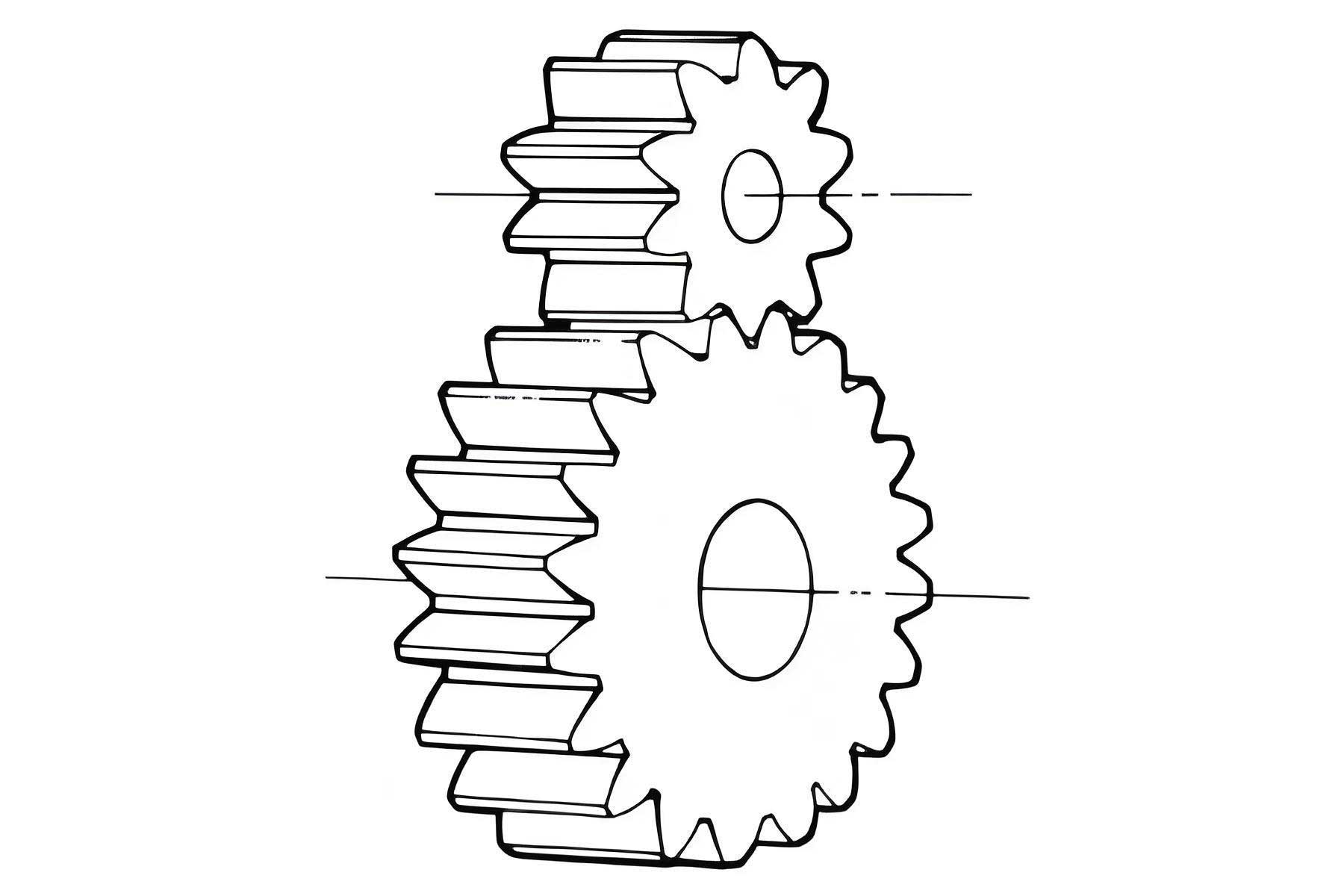
For the root arc segment (ab in Fig. 1), which is generated by the cutter tip, the parametric equations in a coordinate system centered at the gear are given by:
$$ x = r_f \cos \phi, \quad y = r_f \sin \phi $$
where \( r_f \) is the root radius, and \( \phi \) ranges from 0 to \( \theta_b \), with \( \theta_b \) being the angle at the intersection with the transition curve. The tip arc segment (de) is similarly expressed as:
$$ x = r_a \cos \phi, \quad y = r_a \sin \phi $$
where \( r_a \) is the tip radius, and \( \phi \) ranges from \( \theta_d \) to \( \pi/z \), with \( z \) as the number of teeth. The involute curve segment (cd), which forms the active flank of the spur gear, is described by:
$$ x = r_k \cos \phi, \quad y = r_k \sin \phi $$
$$ \text{with} \quad r_k = \frac{r_b}{\cos \alpha_k}, \quad \text{and} \quad \text{inv} \alpha_k = \tan \alpha_k – \alpha_k = \frac{s_b}{2r_b} + \text{inv} \alpha – \phi $$
Here, \( r_b \) is the base radius, \( \alpha_k \) is the pressure angle at point k, \( s_b \) is the base tooth thickness, and \( \alpha \) is the standard pressure angle (typically 20°). The transition curve segment (bc), often neglected or approximated, is critical for stress analysis. For a standard rack cutter with tip radius \( \rho_f \), the transition curve is an extended epicycloid. Its parametric equations are:
$$ x = r_h \left[ \sin(\gamma + \phi) – \frac{\phi}{\cos \gamma} \cos(\gamma + \phi) \right] – \rho_f \sin S, \quad y = r_h \left[ \cos(\gamma + \phi) + \frac{\phi}{\cos \gamma} \sin(\gamma + \phi) \right] + \rho_f \cos S $$
$$ \text{where} \quad S = \frac{H_f}{\rho_f} + \gamma, \quad \gamma = \arctan \left( \frac{\rho_f (1 – \sin \alpha)}{r_h \cos \alpha} \right) $$
In these equations, \( r_h \) is the pitch radius, \( H_f \) is the cutter addendum, and \( \gamma \) is an auxiliary angle. This precise modeling ensures that the spur gear tooth profile is accurately captured, leading to more reliable deformation calculations compared to simplified圆弧 approximations.
To compute the deformation of spur gear teeth under load, we employ Weber’s energy method, which treats the tooth as a variable-section cantilever beam on an elastic foundation. The total deformation at a point j on the tooth flank, where a load \( F_j \) is applied at an angle \( \beta_j \), consists of three components: bending and shear deformation of the cantilever, additional deformation due to foundation elasticity, and contact deformation at the meshing point. This approach is particularly suited for spur gears because it allows for analytical integration with dynamic models.
The bending and shear deformation component \( \delta_{Bj} \) is derived by discretizing the tooth from the load point to the root into small segments i, each with thickness \( T_i \), area \( A_i \), moment of inertia \( I_i \), and distance \( L_{ij} \) to the load point. For a segment i, the contribution to deformation in the direction of \( F_j \) is:
$$ \delta_{Bij} = \frac{F_j}{E_e} \left[ \frac{T_i (T_i^2 + 3L_{ij}^2) \cos^2 \beta_j}{3I_i} + \frac{(2 + 2\nu) T_i \cos^2 \beta_j}{A_i} + \frac{12(1+\nu) T_i \sin^2 \beta_j}{5A_i} \right] $$
where \( E_e \) is the effective elastic modulus, and \( \nu \) is Poisson’s ratio. The effective modulus depends on the gear geometry: for wide spur gears (where tooth width B is greater than five times the pitch tooth thickness \( H_p \)), plane strain conditions apply, so \( E_e = E/(1-\nu^2) \); for narrow spur gears, plane stress conditions apply, so \( E_e = E \), with E being the material’s elastic modulus. Summing over all segments from i=1 to n gives the total bending and shear deformation:
$$ \delta_{Bj} = \sum_{i=1}^{n} \delta_{Bij} $$
The additional deformation due to foundation elasticity \( \delta_{Mj} \) accounts for the flexibility of the gear body. For narrow spur gears, based on R.W. Cornell’s analysis, it is expressed as:
$$ \delta_{Mj} = \frac{F_j \cos^2 \beta_j}{B E H_f^2} \left[ 5.306 \left( \frac{L_f}{H_f} \right)^2 + 2(1+\nu) \left( \frac{L_f}{H_f} \right) + 0.4167 \tan^2 \beta_j + 1.534(1+\nu) \right] $$
where \( L_f = y_j – (x_M – x_j) \tan \beta_j \), with \( x_j, y_j \) being coordinates of point j, and \( x_M, y_M \) defining the critical section at the tooth root. For wide spur gears, under plane strain, the formula adjusts to:
$$ \delta_{Mj} = \frac{F_j \cos^2 \beta_j (1-\nu^2)}{B E H_f^2} \left[ 5.306 \left( \frac{L_f}{H_f} \right)^2 + \frac{2(1-\nu-\nu^2)}{1-\nu^2} \left( \frac{L_f}{H_f} \right) + 0.4167 \tan^2 \beta_j + 1.534 \left(1+\frac{\nu}{1-\nu}\right) \right] $$
The contact deformation \( \delta_{Cj} \) at the meshing point, due to Hertzian contact, is given by:
$$ \delta_{Cj} = \frac{1.275}{E^{0.9} B^{0.8} F_j^{0.1}} $$
Thus, the total deformation \( \delta_j \) at point j for a spur gear tooth pair is the sum of these components:
$$ \delta_j = \delta_{Bj} + \delta_{Mj} + \delta_{Cj} $$
This comprehensive model allows us to compute the deformation across the entire meshing cycle of spur gears. To implement this numerically, we developed a step-by-step computational procedure using Matlab, which efficiently handles the geometric modeling and deformation integration. The flowchart of the process is as follows:
| Step | Description |
|---|---|
| 1 | Input spur gear parameters: number of teeth, module, pressure angle, material properties (E, ν), load, and tooth width. |
| 2 | Compute tooth profile coordinates using the parametric equations for root arc, transition curve, involute, and tip arc. |
| 3 | Determine the meshing points along the tooth profile for a given contact ratio. |
| 4 | Discretize the tooth into small segments from each meshing point to the root. |
| 5 | Calculate bending, shear, foundation, and contact deformations using Weber’s formulas. |
| 6 | Sum the deformations to obtain total deformation at each meshing point. |
| 7 | Output results: deformation curves and meshing stiffness. |
For illustration, we applied this method to a spur gear pair with the following parameters: teeth number z1 = z2 = 28, module m = 3 mm, tooth width B = 10 mm, applied load F_j = 1 N, elastic modulus E = 210 GPa, and Poisson’s ratio ν = 0.3. The spur gears are standard with a pressure angle of 20°. The deformation was calculated at multiple points along the tooth profile during meshing. The results show that as the contact point moves from the root to the tip on the driving spur gear, the deformation increases gradually; conversely, on the driven spur gear, deformation decreases as the contact moves from tip to root. This behavior is consistent with the varying leverage arm and tooth geometry in spur gears.
The single-tooth meshing stiffness, which is the reciprocal of the total deformation per unit load, was also derived. For a spur gear pair, the stiffness varies cyclically during engagement, affecting dynamic response. Our calculations yield a stiffness curve that can be used in dynamic models to predict vibrations. The deformation results for the example spur gears are summarized below:
| Meshing Point Position | Deformation on Driving Spur Gear (μm) | Deformation on Driven Spur Gear (μm) | Total Deformation (μm) |
|---|---|---|---|
| Near root (start) | 0.85 | 1.20 | 2.05 |
| Mid-point | 1.10 | 0.95 | 2.05 |
| Near tip (end) | 1.40 | 0.65 | 2.05 |
These values highlight how deformation shifts between teeth in a spur gear pair. The meshing stiffness K can be computed as \( K = F_j / \delta_j \). For instance, at the start of meshing, \( K \approx 1 / 2.05 \times 10^{-6} = 0.488 \times 10^6 \, \text{N/m} \). The stiffness curve over the meshing cycle shows a smooth transition, with minimum stiffness near the pitch point due to higher deformations. This information is vital for designing spur gear systems to avoid resonance and reduce noise.
The advantages of our method are manifold. First, the precise tooth profile model eliminates errors from圆弧 approximations of the transition curve, which is common in simpler models. This leads to more accurate stress and deformation predictions, especially in the root region where fatigue cracks often initiate in spur gears. Second, Weber’s energy method provides a closed-form solution that is computationally efficient compared to FEA, making it suitable for iterative design processes and integration with system-level dynamics. Third, the Matlab implementation automates the calculation, allowing for rapid analysis of different spur gear geometries and loads. This is particularly useful for optimizing spur gear designs in applications such as automotive transmissions, wind turbines, and industrial machinery.
In conclusion, we have presented a robust numerical framework for calculating tooth deformation in spur gears based on a precise profile model and Weber’s energy method. This approach combines accuracy with computational efficiency, enabling detailed analysis of spur gear meshing stiffness. Future work could extend this to helical gears or incorporate nonlinear effects like plastic deformation. For now, this method serves as a reliable tool for engineers and researchers working on spur gear dynamics, contributing to improved performance and durability of gear systems.