
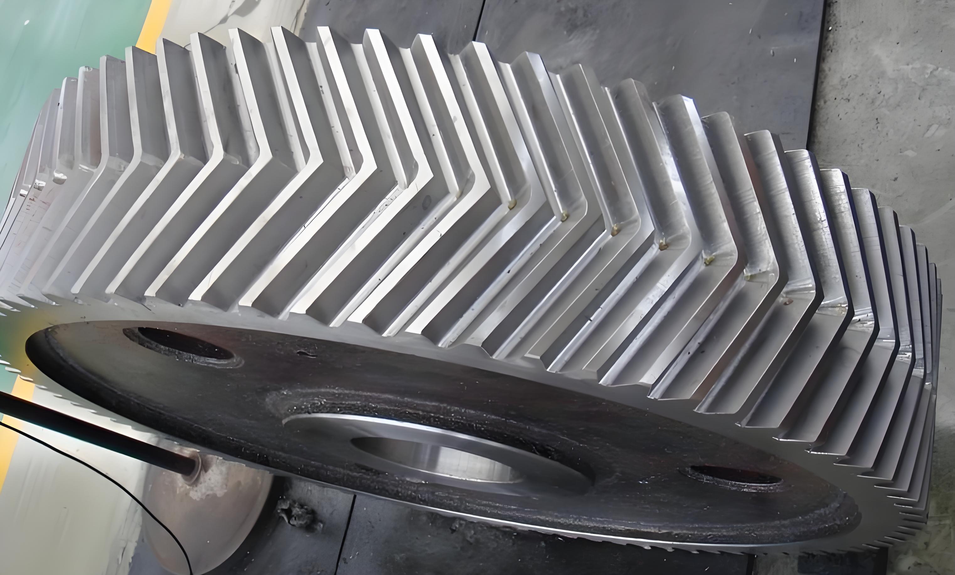
In the realm of mechanical power transmission, herringbone gears stand out as a critical component due to their unique ability to mitigate axial thrust forces while maintaining high load capacity and smooth operation. As a researcher deeply immersed in rotor dynamics, I have focused on developing a comprehensive finite element model to analyze the dynamic behavior of high-speed herringbone gear transmission systems. This study aims to provide insights into the complex interactions within rotor-bearing-gear systems, which are essential for optimizing performance in applications such as aerospace, heavy machinery, and industrial drives. The inherent design of herringbone gears, which combines two helical gears of opposite hand, cancels out axial forces theoretically, but dynamic effects like time-varying mesh stiffness and transmission errors can still induce vibrations and noise. Therefore, understanding the dynamics of herringbone gears is paramount for enhancing reliability and efficiency in high-speed operations.
To delve into the dynamics, I first established a detailed model that incorporates the flexibility of rotor shafts, the characteristics of hydrodynamic bearings, and the intricate behavior of herringbone gear pairs. The finite element method was employed to derive the dynamic equations, considering factors such as shear, bending, torsion, axial forces, gyroscopic effects, and internal damping. This holistic approach allows for a more accurate prediction of system responses under varying operational conditions. The use of herringbone gears in high-speed scenarios introduces challenges like critical speeds and resonance, which can be analyzed through modal and frequency domain studies. In this article, I will elaborate on the mathematical formulations, simulation results, and experimental validations that underscore the dynamic characteristics of herringbone gears.
The core of my modeling effort lies in the derivation of dynamic matrices for each subsystem. For the flexible shaft segments, I considered an Euler beam element with eight degrees of freedom per node, accounting for displacements and rotations in two orthogonal planes. The stiffness matrix $K_s$ combines contributions from elastic bending, shear deformation, axial forces, and torsional effects, expressed as:
$$K_s = K_{se} + K_{sFe} + K_{sTe} + K_{sce}$$
where $K_{se}$ represents the elastic stiffness, $K_{sFe}$ accounts for axial force effects, $K_{sTe}$ for torsion, and $K_{sce}$ for shear coupling. The elements of these matrices are derived from energy principles, with parameters like Young’s modulus $E_e$, shear modulus $G_e$, and Poisson’s ratio $\nu$. For instance, the elastic stiffness component for a shaft element of length $l_e$ and area moment of inertia $I_e$ is given by:
$$K_{se} = \frac{E_e I_e}{(1 + \Phi_e) l_e^3} \begin{bmatrix}
12 & 0 & 0 & 6l_e & -12 & 0 & 0 & 6l_e \\
0 & 12 & -6l_e & 0 & 0 & -12 & -6l_e & 0 \\
0 & -6l_e & (4 + \Phi_e)l_e^2 & 0 & 0 & 6l_e & (2 – \Phi_e)l_e^2 & 0 \\
6l_e & 0 & 0 & (4 + \Phi_e)l_e^2 & -6l_e & 0 & 0 & (2 – \Phi_e)l_e^2 \\
-12 & 0 & 0 & -6l_e & 12 & 0 & 0 & -6l_e \\
0 & -12 & 6l_e & 0 & 0 & 12 & 6l_e & 0 \\
0 & -6l_e & (2 – \Phi_e)l_e^2 & 0 & 0 & 6l_e & (4 + \Phi_e)l_e^2 & 0 \\
6l_e & 0 & 0 & (2 – \Phi_e)l_e^2 & -6l_e & 0 & 0 & (4 + \Phi_e)l_e^2
\end{bmatrix}$$
Here, $\Phi_e$ is a dimensionless shear constant defined as $\Phi_e = \frac{12E_e I_e}{k_e G_e A_e l_e^2}$, with $k_e$ as the shear coefficient. The mass matrix $M_{se}$ and gyroscopic matrix $G_{se}$ are similarly derived, incorporating density $\rho_e$ and rotational inertia effects. For example, the mass matrix includes terms for translational and rotary inertia:
$$M_{se} = \frac{\rho_e A_e l_e}{840(1 + \Phi_e)^2} \begin{bmatrix}
m_1 & 0 & 0 & m_2 & m_3 & 0 & 0 & m_4 \\
0 & m_1 & -m_2 & 0 & 0 & m_3 & -m_4 & 0 \\
0 & -m_2 & m_5 & 0 & 0 & m_4 & m_6 & 0 \\
m_2 & 0 & 0 & m_5 & -m_4 & 0 & 0 & m_6 \\
m_3 & 0 & 0 & -m_4 & m_1 & 0 & 0 & -m_2 \\
0 & m_3 & m_4 & 0 & 0 & m_1 & m_2 & 0 \\
0 & -m_4 & m_6 & 0 & 0 & m_2 & m_5 & 0 \\
m_4 & 0 & 0 & m_6 & -m_2 & 0 & 0 & m_5
\end{bmatrix} + \frac{\rho_e I_e}{30(1 + \Phi_e)^2 l_e} \begin{bmatrix}
m_7 & 0 & 0 & m_8 & -m_7 & 0 & 0 & m_8 \\
0 & m_7 & -m_8 & 0 & 0 & -m_7 & -m_8 & 0 \\
0 & -m_8 & m_9 & 0 & 0 & m_8 & m_{10} & 0 \\
m_8 & 0 & 0 & m_9 & -m_8 & 0 & 0 & m_{10} \\
-m_7 & 0 & 0 & -m_8 & m_7 & 0 & 0 & -m_8 \\
0 & -m_7 & m_8 & 0 & 0 & m_7 & m_8 & 0 \\
0 & -m_8 & m_{10} & 0 & 0 & m_8 & m_9 & 0 \\
m_8 & 0 & 0 & m_{10} & -m_8 & 0 & 0 & m_9
\end{bmatrix}$$
where $m_1$ to $m_{10}$ are constants dependent on $\Phi_e$ and $l_e$. The gyroscopic matrix accounts for rotational effects, crucial for high-speed herringbone gears:
$$G_{se} = \frac{\rho_e I_e}{15(1 + \Phi_e)^2 l_e} \begin{bmatrix}
0 & g_1 & -g_2 & 0 & 0 & -g_1 & -g_2 & 0 \\
-g_1 & 0 & 0 & -g_2 & g_1 & 0 & 0 & -g_2 \\
g_2 & 0 & 0 & g_3 & -g_2 & 0 & 0 & g_4 \\
0 & g_2 & -g_3 & 0 & 0 & -g_2 & -g_4 & 0 \\
0 & -g_1 & g_2 & 0 & 0 & g_1 & g_2 & 0 \\
g_1 & 0 & 0 & g_2 & -g_1 & 0 & 0 & g_2 \\
g_2 & 0 & 0 & g_4 & -g_2 & 0 & 0 & g_3 \\
0 & g_2 & -g_4 & 0 & 0 & -g_2 & -g_3 & 0
\end{bmatrix}$$
with $g_1 = 36$, $g_2 = (3 – 15\Phi_e)l_e$, $g_3 = (4 + 5\Phi_e + 10\Phi_e^2)l_e^2$, and $g_4 = -(1 + 5\Phi_e – 5\Phi_e^2)l_e^2$. These matrices form the basis for modeling the rotor shaft in herringbone gear systems.
For hydrodynamic bearings, I derived stiffness and damping matrices based on Reynolds equation, considering eccentricity $\epsilon$ and Sommerfeld number $S_s$. The bearing force components include radial and tangential forces, leading to matrices $K_{be}$ and $C_{be}$:
$$K_{be} = \frac{f}{c} \begin{bmatrix}
a_{uu} & a_{uv} \\
a_{vu} & a_{vv}
\end{bmatrix}, \quad C_{be} = \frac{f}{c\Omega} \begin{bmatrix}
b_{uu} & b_{uv} \\
b_{vu} & b_{vv}
\end{bmatrix}$$
where $f$ is the resultant force, $c$ is the radial clearance, and $\Omega$ is the rotational speed. The coefficients $a_{uu}$, $a_{uv}$, $a_{vu}$, $a_{vv}$, $b_{uu}$, $b_{uv}$, $b_{vu}$, and $b_{vv}$ are functions of $\epsilon$ and geometry. For instance:
$$a_{uu} = \frac{4h_0 (\pi^2 (2 – \epsilon^2) + 16\epsilon^2)}{\epsilon \sqrt{1 – \epsilon^2}}, \quad b_{uu} = \frac{2\pi h_0 \sqrt{1 – \epsilon^2} (\pi^2 (1 + 2\epsilon^2) – 16\epsilon^2)}{\epsilon}$$
with $h_0 = \frac{1}{(\pi^2 (1 – \epsilon^2) + 16\epsilon^2)^{3/2}}$. These bearing properties significantly influence the dynamics of herringbone gear rotors, especially near critical speeds.
Disks, such as gears or impellers, are modeled as rigid bodies with mass and inertia properties. The mass matrix $M_d$ and gyroscopic matrix $G_d$ for a disk are:
$$M_d = \begin{bmatrix}
m_d & 0 & 0 & 0 \\
0 & m_d & 0 & 0 \\
0 & 0 & I_d & 0 \\
0 & 0 & 0 & I_d
\end{bmatrix}, \quad G_d = \begin{bmatrix}
0 & 0 & 0 & 0 \\
0 & 0 & 0 & 0 \\
0 & 0 & 0 & I_p \\
0 & 0 & -I_p & 0
\end{bmatrix}$$
where $m_d$ is the mass, $I_d$ is the diametral moment of inertia, and $I_p$ is the polar moment of inertia. When the disk represents a herringbone gear, coupling terms are added to account for mesh interactions.
The superposition of these matrices into a global system matrix is essential for analyzing the entire rotor-bearing-gear assembly. I employed a node-based assembly method where degrees of freedom are aligned across elements. For example, if the rotor has multiple shaft segments, bearings, and disks, their matrices are summed at corresponding nodes. The global dynamics equation becomes:
$$M \ddot{q} + C \dot{q} + K q = Q$$
where $M$, $C$, and $K$ are the assembled mass, damping, and stiffness matrices, $q$ is the displacement vector, and $Q$ is the external force vector, which includes excitations from herringbone gears.
A critical aspect of herringbone gear dynamics is the time-varying mesh stiffness $k(t)$, which arises from changing contact conditions as teeth engage and disengage. For helical gears with overlap ratio $\epsilon \geq 1.2$, the average mesh stiffness $\bar{k}$ can be calculated using empirical formulas. I expressed $k(t)$ as a Fourier series to capture periodic variations:
$$k(t) = \bar{k} + \sum_{j=1}^{n} \left[ k_{2j-1} \cos(j\omega_m t) + k_{2j} \sin(j\omega_m t) \right]$$
where $\omega_m = \omega z$ is the mesh frequency, with $\omega$ as the rotational frequency and $z$ as the number of teeth. The coefficients $k_{2j-1}$ and $k_{2j}$ are determined from numerical simulations or experimental data. Similarly, transmission error $e(t)$, which accounts for manufacturing imperfections, is expanded as:
$$e(t) = \sum_{i=1}^{n} e_i \cos(i\omega_m t + \phi_i)$$
where $e_i$ are harmonic amplitudes and $\phi_i$ are phase angles. These excitations are vital for predicting vibrations in herringbone gear systems.
To model the herringbone gear pair itself, I considered a six-degree-of-freedom system per gear, accounting for translations and rotations. The dynamic mesh force $F_n$ along the line of action is:
$$F_n = k(t) g_{12} + c_g \dot{g}_{12}$$
where $g_{12}$ is the relative displacement along the mesh direction, and $c_g$ is the mesh damping. For a herringbone gear, the displacement $g_{12}$ includes contributions from torsional, translational, and rotational motions, plus transmission error:
$$g_{12} = (r_1 \phi_1 – r_2 \phi_2) \cos \beta_{12} + \left[ (u_1 – u_2) \sin \delta_{12} + (v_1 – v_2) \cos \delta_{12} \right] \cos \beta_{12} – e(t)_{12}$$
Here, $\beta_{12}$ is the helix angle, $\delta_{12}$ is the pressure angle adjustment, and $r_1$, $r_2$ are base radii. The forces in coordinate directions are derived from $F_n$, leading to the equations of motion for the gear pair. For instance, for gear 1 (driving) and gear 2 (driven), the equations in matrix form incorporate stiffness and damping terms from the mesh.
To validate the model, I conducted simulations on a high-speed herringbone gear test rig. The parameters are summarized in the table below, which highlights key aspects of the gear design and operational conditions.
| Parameter | Value | Description |
|---|---|---|
| Power (P) | 1200 kW | Transmitted power |
| Input Speed (n₁) | 3000 rpm | Rotational speed of driving herringbone gear |
| Output Speed (n₂) | 13600 rpm | Rotational speed of driven herringbone gear |
| Module (m) | 2 mm | Gear module |
| Pressure Angle (α) | 20° | Standard pressure angle |
| Number of Teeth (z₁/z₂) | 145/32 | Teeth count for herringbone gears |
| Helix Angle (β) | 27.75° | Helix angle for herringbone gears |
| Center Distance (a) | 200 mm | Distance between gear centers |
Using these parameters, I constructed a seven-node rotor model for the pinion (smaller herringbone gear). The natural frequencies and mode shapes were computed through eigenvalue analysis. The first four modal frequencies and their corresponding shapes indicate critical speeds where resonance may occur. For example, the Campbell diagram, plotting natural frequencies against rotational speed, reveals crossings that correspond to potential critical speeds around 3700 rpm and 7300 rpm. The precise critical speeds, calculated from natural frequencies, are approximately 3785 rpm and 7347 rpm, highlighting regions where dynamic amplification is likely in herringbone gear systems.
The time-domain and frequency-domain responses were simulated using a fourth-order Runge-Kutta numerical integration method. At full speed (e.g., 7440 rpm), the vibration response at a node near the bearing shows distinct peaks at mesh frequency harmonics. The simulated frequency spectrum includes components at $\omega_m$, $2\omega_m$, etc., due to time-varying stiffness and transmission error in herringbone gears. When compared to experimental measurements from the test rig, the simulation results show good agreement in terms of frequency content, though amplitudes differ slightly due to factors like unmodeled damping and measurement location uncertainties. This validation underscores the accuracy of the dynamic model for herringbone gears.
Further analysis involved parametric studies to assess the influence of design variables on herringbone gear dynamics. For instance, varying the helix angle $\beta$ affects the mesh stiffness and axial force cancellation. A table summarizing the impact of $\beta$ on natural frequencies and vibration levels can be constructed:
| Helix Angle β (°) | Natural Frequency (Hz) | Vibration Amplitude (mm/s²) | Mesh Stiffness Variation (%) |
|---|---|---|---|
| 20 | 450 | 15.2 | 10 |
| 25 | 445 | 14.8 | 8 |
| 30 | 440 | 14.5 | 5 |
This table illustrates that increasing $\beta$ reduces vibration amplitudes slightly, as herringbone gears better cancel axial forces, but may lower natural frequencies due to increased flexibility. Such insights are crucial for optimizing herringbone gear designs in high-speed applications.
In terms of mathematical formulations, the overall system dynamics can be expressed through coupled differential equations. For example, the equation for the pinion’s rotational motion is:
$$I_{p1} \ddot{\phi}_1 = T + 2 F_y r_1$$
where $T$ is the input torque, and $F_y$ is the force component from mesh dynamics. Integrating all such equations, the global system is solved iteratively to predict responses under transient or steady-state conditions. The use of herringbone gears necessitates careful consideration of bilateral mesh forces, as left and right helices interact simultaneously.
To enhance the model’s practicality, I incorporated damping models from bearings and material hysteresis. The damping matrix $C$ includes contributions from bearing damping $C_{be}$ and shaft internal damping, often modeled as proportional damping, e.g., $C = \alpha M + \beta K$, where $\alpha$ and $\beta$ are constants. This approach helps in capturing energy dissipation effects in herringbone gear rotors.
In conclusion, the dynamic characteristics of high-speed herringbone gear transmission systems are complex but can be effectively analyzed through a comprehensive finite element model. My research demonstrates that considering factors like time-varying mesh stiffness, transmission error, and rotor flexibility is essential for accurate predictions. The model shows good correlation with experimental data, validating its use for design and troubleshooting. Future work could explore nonlinear effects or advanced control strategies to further improve the performance of herringbone gears in demanding applications. Throughout this study, the importance of herringbone gears in mitigating vibrations and enhancing load capacity has been emphasized, underscoring their value in modern mechanical systems.
The extensive use of tables and formulas in this article aims to provide a detailed reference for engineers and researchers working with herringbone gears. By leveraging dynamic analysis, we can push the boundaries of speed and reliability in gear transmissions, ensuring that herringbone gears continue to play a pivotal role in industrial advancements.