
As the core component of mechanical equipment, the performance of transmission systems directly affects the operational efficiency and service life of the entire machinery. Among the numerous transmission systems, the variable-speed transmission, serving as the key device for converting different rotational speeds and torques, has always been a research hotspot in the field of mechanical engineering. The novel bevel gear-roller plate transmission, as a transmission device characterized by high efficiency and stability, provides a new solution for modern industrial transmission systems with its unique structural design and transmission mechanism. However, in practical applications, due to the complex and variable working environment, traditional control methods often struggle to guarantee the stability and precision of constant speed output from the transmission. Therefore, researching an adaptive control method capable of achieving constant speed output is particularly important.
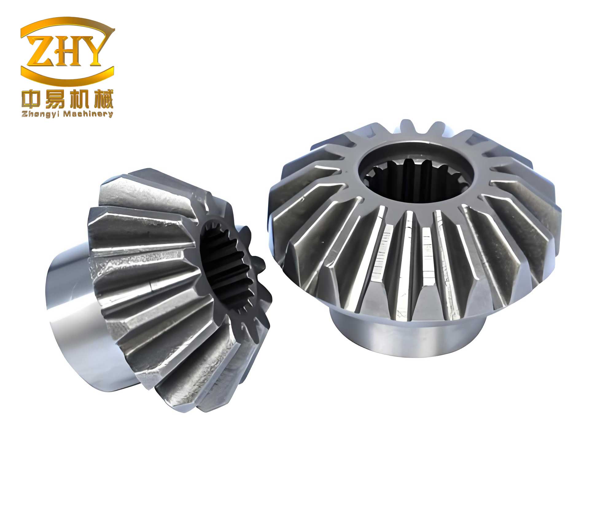
This paper focuses on a novel bevel gear-roller plate transmission system. Its nonlinear characteristics and operational uncertainties pose significant challenges to maintaining a constant output shaft speed under varying loads. To address this, a dedicated Fuzzy PID control strategy is proposed. The strategy begins with a detailed dynamic modeling of the transmission, followed by the design of a Fuzzy PID controller. The controller dynamically adjusts the parameters of a conventional PID controller based on real-time system error and its rate of change. Finally, the control signal is calculated and applied to the transmission’s actuator to regulate the input, thereby achieving constant output speed.
1. Dynamic Modeling of the Novel Bevel Gear-Roller Plate Transmission
The novel transmission combines a bevel gear set with a roller-plate continuous variable mechanism. The bevel gear section is responsible for providing a base speed ratio, while the roller-plate section enables fine, continuous speed adjustment. Accurate dynamic modeling is the foundation for effective control system design. The modeling integrates the kinematics and dynamics of both the bevel gears and the roller-plate assembly, considering factors like load influence on the effective gear ratio and frictional losses in the roller-plate contact.
1.1 Modeling of the Bevel Gear Section
The input and output speeds of the bevel gear set are related by its gear ratio. However, in a real system under load, the effective transmission ratio can be influenced by factors like shaft deflection and tooth deformation. To account for this, a load-dependent coefficient $k_L$ is introduced. Let $\omega_{in}$ and $\omega_{out}$ be the input and output shaft angular velocities, respectively, and $N_1$ and $N_2$ be the number of teeth on the driving and driven bevel gears. The effective gear ratio $i$ is given by:
$$ i = \frac{\omega_{in}}{\omega_{out}} = \frac{N_1}{N_2} \cdot k_L(T_{out}) $$
Here, $k_L(T_{out})$ is a nonlinear function of the output torque $T_{out}$, representing the load’s effect on the ratio. For simplification in control design, it can often be approximated by a linear or low-order polynomial function based on experimental data.
1.2 Modeling of the Roller-Plate Section
The roller-plate mechanism transmits torque through friction. The primary resisting torque in this section is the rolling resistance moment $M_r$. This moment depends on the normal force $F_n$ between the roller and plate, the coefficient of friction $\mu$, the roller’s linear velocity $v$, angular acceleration $\alpha$, material properties (density $\rho$), and geometric parameters like roller radius $R$. A comprehensive model can be complex; a practical representation often uses a rolling resistance coefficient $f_r$ that encapsulates many of these effects. The rolling resistance moment can be expressed as a function:
$$ M_r = f_r(v, \alpha, F_n, \mu, \rho, R, \ldots) $$
For controller design, a simplified model such as $M_r = C_{rr} \cdot F_n \cdot R$ is often used, where $C_{rr}$ is an empirical rolling resistance coefficient, though more detailed models improve accuracy.
1.3 Integrated Dynamic Equation
Combining the dynamics of both sections and applying Newton’s second law for rotation to the output shaft yields the integrated dynamic equation of the transmission:
$$ \frac{T_{in}}{i} – T_{out} = J_{out} \cdot \frac{d\omega_{out}}{dt} + M_r $$
Where:
- $T_{in}$ is the input torque.
- $T_{out}$ is the output load torque.
- $J_{out}$ is the moment of inertia of the output shaft and its connected load.
- $\frac{d\omega_{out}}{dt}$ is the angular acceleration of the output shaft.
This equation forms the fundamental plant model for designing the speed controller. The control objective is to manipulate $T_{in}$ (or $\omega_{in}$) such that $\omega_{out}$ tracks a desired constant reference value $\omega_{ref}$ despite variations in $T_{out}$ and other internal disturbances represented by $M_r$.
2. Fuzzy PID Controller Design for Constant Speed Output
Proportional-Integral-Derivative (PID) control is ubiquitous in industry due to its simplicity. However, its fixed parameters struggle with the nonlinearities and parameter variations present in the bevel gear-roller plate transmission. Fuzzy logic provides a method to adjust these parameters in real-time based on the system’s operating state. The designed Fuzzy PID controller uses the output speed error and its derivative as inputs to a fuzzy inference system (FIS) which outputs adjustments for the PID gains.
2.1 Controller Structure and Input Selection
The structure of the proposed control system is shown in the block diagram below (conceptually). The core is a conventional PID controller whose parameters $(K_p, K_i, K_d)$ are dynamically modified by a fuzzy inference module. The inputs to this fuzzy module are:
- Speed Error (e): The difference between the desired reference speed and the measured output speed.
$$ e(k) = \omega_{ref} – \omega_{out}(k) $$ - Change of Error (ec or $\Delta e$): The rate at which the error is changing, approximated by the difference between consecutive errors.
$$ ec(k) = \frac{e(k) – e(k-1)}{\Delta t} \approx \Delta e(k) $$
These two signals comprehensively describe the system’s deviation from the setpoint and its trend.
2.2 Fuzzification and Membership Functions
The crisp inputs $e$ and $ec$ are mapped to fuzzy linguistic variables. For both inputs and the output gains, seven fuzzy sets are typically defined: Negative Big (NB), Negative Medium (NM), Negative Small (NS), Zero (Z), Positive Small (PS), Positive Medium (PM), Positive Big (PB). The universe of discourse for $e$ and $ec$ must be scaled from their physical ranges $[-E, E]$ and $[-EC, EC]$ to a normalized range $[-n, n]$ and $[-m, m]$ using quantization factors $k_e$ and $k_{ec}$:
$$ k_e = \frac{n}{E}, \quad k_{ec} = \frac{m}{EC} $$
Triangular or Gaussian membership functions are commonly used to define the degree of membership for each fuzzy set. An example for the error input is conceptually described in Table 1.
| Fuzzy Set | Linguistic Meaning | Typical Normalized Range |
|---|---|---|
| NB | Negative Big | [-1.0, -0.6] |
| NM | Negative Medium | [-0.8, -0.3] |
| NS | Negative Small | [-0.5, 0] |
| Z | Zero | [-0.2, 0.2] |
| PS | Positive Small | [0, 0.5] |
| PM | Positive Medium | [0.3, 0.8] |
| PB | Positive Big | [0.6, 1.0] |
2.3 Fuzzy Rule Base and Inference
The heart of the fuzzy tuner is the rule base, which encapsulates expert knowledge on how to adjust PID gains based on $e$ and $ec$. The rules are of the form: IF $e$ is A AND $ec$ is B, THEN $\Delta K_p$ is C, $\Delta K_i$ is D, $\Delta K_d$ is E. A typical rule base for $\Delta K_p$ adjustment is shown in Table 2. For example, if the error is large and positive (PB) and not changing fast (Z), a large increase in $K_p$ (PB) is needed to quickly reduce the error. Conversely, if the error is small but increasing rapidly (PS and PB for ec), a moderate increase in $K_d$ (PM) might be warranted to dampen the change.
| e \ ec | NB | NM | NS | Z | PS | PM | PB |
|---|---|---|---|---|---|---|---|
| NB | PB | PB | PM | PM | PS | Z | Z |
| NM | PB | PB | PM | PS | PS | Z | NS |
| NS | PM | PM | PS | PS | Z | NS | NS |
| Z | PM | PM | PS | Z | NS | NM | NM |
| PS | PS | PS | Z | NS | NS | NM | NM |
| PM | PS | Z | NS | NM | NM | NM | NB |
| PB | Z | Z | NM | NM | NM | NB | NB |
Separate but analogous rule tables are constructed for $\Delta K_i$ and $\Delta K_d$. The fuzzy inference engine (using, e.g., Mamdani type) evaluates all rules that are “fired” given the current crisp inputs, combining their outputs to produce fuzzy sets for $\Delta K_p$, $\Delta K_i$, and $\Delta K_d$.
2.4 Defuzzification and PID Parameter Update
The resulting fuzzy output sets need to be converted back into crisp numerical values to adjust the PID gains. The Center of Gravity (COG) or Weighted Average method is commonly used for defuzzification. For an output variable $\Delta K$ with membership function $\mu_{\Delta K}(x)$ over discrete universe $X = \{x_1, x_2, …, x_q\}$, the crisp output is:
$$ \Delta K = \frac{\sum_{j=1}^{q} x_j \cdot \mu_{\Delta K}(x_j)}{\sum_{j=1}^{q} \mu_{\Delta K}(x_j)} $$
This process yields the real-time adjustments $\Delta K_p(k)$, $\Delta K_i(k)$, and $\Delta K_d(k)$. The PID controller parameters are then updated at each sample time $k$:
$$ K_p(k) = K_{p0} + \Delta K_p(k) $$
$$ K_i(k) = K_{i0} + \Delta K_i(k) $$
$$ K_d(k) = K_{d0} + \Delta K_d(k) $$
where $K_{p0}$, $K_{i0}$, $K_{d0}$ are the initial or baseline PID parameters.
2.5 Final Control Signal Calculation
Finally, the PID controller computes the control signal $u(t)$ (which typically corresponds to a command for input torque $T_{in}$ or a related actuator) using the updated gains:
$$ u(t) = K_p(t) \cdot e(t) + K_i(t) \cdot \int_0^t e(\tau) d\tau + K_d(t) \cdot \frac{de(t)}{dt} $$
This signal is then sent to the transmission’s power source or actuator to regulate the input, closing the loop and driving the output speed $\omega_{out}$ towards the constant reference $\omega_{ref}$.
3. Simulation Analysis and Discussion
To validate the effectiveness of the proposed Fuzzy PID control strategy for the bevel gear-roller plate transmission, a comparative simulation study was conducted. The transmission model was implemented in a simulation environment (e.g., MATLAB/Simulink) using parameters representative of a mid-range automotive or industrial application. Key parameters of the simulated transmission model are summarized in Table 3.
| Parameter | Symbol | Value | Unit |
|---|---|---|---|
| Driving Bevel Gear Teeth | $N_1$ | 24 | – |
| Driven Bevel Gear Teeth | $N_2$ | 48 | – |
| Base Gear Ratio | $N_1/N_2$ | 0.5 | – |
| Roller Radius | $R_r$ | 0.05 | m |
| Plate Contact Radius (max) | $R_p$ | 0.15 | m |
| Output Shaft Inertia | $J_{out}$ | 0.25 | kg·m² |
| Rolling Resistance Coefficient | $C_{rr}$ | 0.012 | – |
| Reference Output Speed | $\omega_{ref}$ | 150 | rad/s |
3.1 Control Performance under Load Torque Variation
The primary test was to maintain a constant output speed of 150 rad/s while subjecting the transmission to a step change in output load torque. The load torque $T_{out}$ was initially 50 N·m and stepped up to 150 N·m at time t = 5 seconds. The performance of the proposed Fuzzy PID controller was compared against a conventional fixed-gain PID controller, which was tuned for best performance at the nominal load. The simulation results for output speed are shown conceptually.
The Fuzzy PID controller demonstrated superior performance:
- Reduced Overshoot: Upon the load increase, the fixed PID controller exhibited a significant speed drop followed by an overshoot during recovery. The Fuzzy PID controller minimized this overshoot, leading to a smoother recovery.
- Faster Settling Time: The Fuzzy PID controller brought the speed back to the reference value more quickly after the disturbance.
- Steady-State Accuracy: Both controllers eliminated steady-state error due to the integral action, but the Fuzzy PID maintained marginally smaller error bounds during the transient.
The adaptive nature of the Fuzzy PID allowed it to increase the proportional and integral gains appropriately when a large error occurred due to the load step, resulting in a more aggressive corrective action. Simultaneously, it adjusted the derivative gain to prevent excessive oscillation.
3.2 Quantitative Performance Metrics
The performance was quantitatively evaluated using standard metrics: Maximum Overshoot ($M_p$), Settling Time ($T_s$, to within ±2% of reference), and Integral of Absolute Error (IAE). The results for the load step scenario are summarized in Table 4.
| Control Method | Max Overshoot $M_p$ (%) | Settling Time $T_s$ (s) | IAE (rad) |
|---|---|---|---|
| Fixed PID | 4.8 | 1.8 | 15.2 |
| Fuzzy PID (Proposed) | 1.2 | 1.1 | 8.7 |
The table clearly indicates the advantages of the proposed method across all metrics, with overshoot reduced by approximately 75% and settling time improved by nearly 40%.
3.3 Robustness to Parameter Variation
A secondary test evaluated robustness. The moment of inertia $J_{out}$ was increased by 30% from its nominal value to simulate a change in the driven load. The fixed PID controller, tuned for the nominal inertia, showed increased oscillation and a longer settling time. In contrast, the Fuzzy PID controller automatically compensated for this change, maintaining performance metrics close to those achieved with the nominal parameters. This demonstrates the inherent robustness provided by the fuzzy adaptation mechanism to variations within the plant model, a common occurrence in systems involving bevel gears and friction-dependent components.
4. Conclusion
This paper presented a Fuzzy PID control strategy for achieving constant speed output in a novel bevel gear-roller plate transmission. The dynamic model of the transmission incorporated the load-influenced gear ratio of the bevel gears and the rolling resistance of the continuous variable unit, providing a realistic basis for controller design. The core of the strategy is a fuzzy inference system that dynamically adjusts the proportional, integral, and derivative gains of a PID controller based on the real-time speed error and its rate of change.
Simulation studies confirmed the effectiveness of the proposed method. Compared to a conventional fixed-gain PID controller, the Fuzzy PID controller demonstrated significantly improved performance when rejecting load disturbances: it achieved markedly lower overshoot, faster settling time, and reduced integral error. Furthermore, it exhibited greater robustness to variations in system parameters such as load inertia.
The integration of fuzzy logic with classical PID control offers a practical and powerful solution for managing the nonlinearities and uncertainties inherent in complex mechanical transmissions like the one studied. The method enhances system adaptability and stability without requiring an excessively complex mathematical model of the plant. Future work could explore the implementation of this algorithm on real-time hardware, experimental validation on a physical prototype, and potential extension to more advanced fuzzy or neuro-fuzzy architectures for even more challenging operational scenarios.