Analysis of Roller Rotational Speed in Single Cylindrical Roller Enveloping Worm Drive

The pursuit of higher efficiency and greater load capacity in power transmission systems has been a constant driver of innovation within mechanical engineering. Among the various gear types, the worm gear set, or screw gear drive, occupies a crucial niche, offering high reduction ratios and compact design in a single stage. However, the traditional design, relying on direct sliding contact between the helical thread of the worm and the conjugate tooth surface of the wheel, is inherently limited by significant sliding friction. This friction leads to reduced transmission efficiency, notable energy losses in the form of heat, and accelerated wear of the contacting surfaces, ultimately constraining the power density and service life of the assembly. To fundamentally address these limitations, a novel configuration has been developed: the roller enveloping worm drive. In this design, the traditional teeth on the worm wheel are replaced by an array of cylindrical rollers (or pins). Theoretically, this substitution aims to transform the predominant sliding friction at the mesh into rolling friction, thereby promising a substantial leap in efficiency and durability for this type of screw gear transmission. My investigation focuses specifically on the kinematics of a single cylindrical roller within such a system, analyzing its complex motion during engagement to determine its instantaneous rotational speed, a parameter critical to realizing the promised performance benefits.

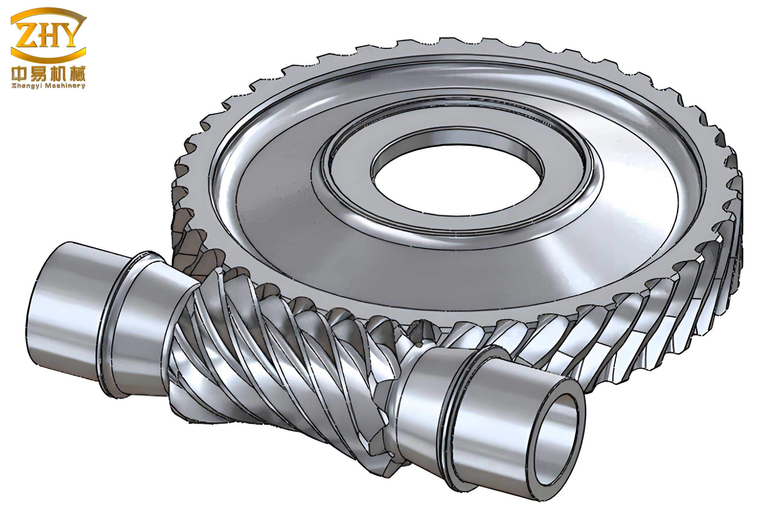
The primary motivation for this study stems from observations in prototype testing of roller enveloping worm drives. While the theoretical efficiency gains are compelling, practical implementations often fall short of expectations. A key issue identified is the non-fluent, often inconsistent rotation of the worm wheel rollers. Instead of pure, unhindered rolling, the rollers exhibit erratic self-rotation or even partial locking, which reintroduces sliding components and negates the efficiency advantage. This phenomenon suggests that the kinematics of the roller are more complex than a simple conversion of worm translation into roller rotation. Therefore, a precise understanding of the instantaneous rotational speed of a roller, and how it varies during the engagement cycle, is not merely an academic exercise but a necessary step for optimizing the geometry, minimizing internal sliding, and unlocking the full potential of this advanced screw gear concept.

1. Geometrical Model and Coordinate Systems of the Single Roller Enveloping Worm Drive

To establish a rigorous foundation for the kinematic analysis, we begin by defining a complete set of coordinate systems that describe the spatial relationship between the worm, the worm wheel (gear), and the single cylindrical roller under investigation. This mathematical framework is essential for applying the principles of gearing theory and differential geometry. The worm is a globoid (hourglass) type that envelopes the roller. The following coordinate systems are established, as illustrated in the conceptual diagram:

Fixed Global Frames: Two stationary coordinate systems are defined. The system $\sigma_1′(O_1′ – \mathbf{i}_1′, \mathbf{j}_1′, \mathbf{k}_1′)$ is attached to the machine frame with its origin at the theoretical center of the worm shaft. Similarly, $\sigma_2′(O_2′ – \mathbf{i}_2′, \mathbf{j}_2′, \mathbf{k}_2′)$ is fixed with its origin at the theoretical center of the worm wheel shaft. The axes $\mathbf{k}_1’$ and $\mathbf{k}_2’$ are collinear with the rotational axes of the worm and the gear, respectively. These two axes are perpendicular and separated by the central distance, denoted by $a$.
Moving Body Frames: Two frames rotate with their respective components. Frame $\sigma_1(O_1 – \mathbf{i}_1, \mathbf{j}_1, \mathbf{k}_1)$ is rigidly attached to the worm, rotating with it about the $\mathbf{k}_1’$ axis by an angle $\varphi_1$. Frame $\sigma_2(O_2 – \mathbf{i}_2, \mathbf{j}_2, \mathbf{k}_2)$ is rigidly attached to the worm wheel, rotating with it about the $\mathbf{k}_2’$ axis by an angle $\varphi_2$. At the initial position $(\varphi_1 = \varphi_2 = 0)$, the moving frames coincide with their corresponding fixed frames. The relationship between the rotation angles is governed by the gear ratio $i_{12}$: $\varphi_1 = i_{12} \cdot \varphi_2$. For a single-start worm, $i_{12}$ equals the number of teeth on the gear, $z_2$.
Roller Frame: A coordinate system $\sigma_0(O_0 – \mathbf{i}_0, \mathbf{j}_0, \mathbf{k}_0)$ is defined for the cylindrical roller. Its origin $O_0$ is placed at the center of one end (the “top”) of the roller. The axis $\mathbf{k}_0$ is aligned with the axis of the roller cylinder, which is radial relative to the worm wheel and perpendicular to the wheel’s axis $\mathbf{k}_2’$. Within the worm wheel frame $\sigma_2$, the coordinates of $O_0$ are $(x_0^{(2)}, y_0^{(2)}, z_0^{(2)})$. From the assembly geometry, $y_0^{(2)} = z_0^{(2)} = 0$ and $x_0^{(2)} = r_{a2}$, where $r_{a2}$ is the radial distance from the worm wheel axis to the roller axis (the pitch radius of the roller circle).
Contact Point Frame (Moving Trihedron): For analyzing conditions at the point of contact, a local frame $\sigma_p(O_p – \mathbf{e}_1, \mathbf{e}_2, \mathbf{n})$ is defined directly on the roller surface at the instantaneous contact point $P$. Here, $\mathbf{n}$ is the unit normal vector to the roller surface at $P$, $\mathbf{e}_1$ is the unit vector in the circumferential (tangential) direction of the roller, and $\mathbf{e}_2$ is the unit vector along the roller’s axis ($\mathbf{k}_0$).

The surface of the cylindrical roller is defined in its own frame $\sigma_0$ by the vector equation:
$$\mathbf{r}_0 = x_0 \mathbf{i}_0 + y_0 \mathbf{j}_0 + z_0 \mathbf{k}_0$$
with the parametric equations:
$$
\begin{aligned}
x_0 &= R \cos \theta, \\
y_0 &= R \sin \theta, \\
z_0 &= u.
\end{aligned}
$$
Here, $R$ is the radius of the roller, $\theta$ is the angular parameter measured from the $\mathbf{i}_0$ axis around the roller’s circumference, and $u$ is the axial parameter along the roller’s length ($\mathbf{k}_0$ direction). This parameterization is fundamental for describing the locus of potential contact points.

2. Kinematic Analysis: Relative Velocity at the Contact Point

The core of the kinematic investigation lies in determining the relative velocity between the worm surface and the roller surface at their instantaneous point of contact, $P$. According to the fundamental theory of gearing, this relative velocity vector, denoted $\mathbf{v}^{(12)}$, lies in the common tangent plane at $P$ and is key to understanding the sliding and rolling conditions. It is derived from the general relative motion formula:

$$\mathbf{v}^{(12)} = \frac{d\boldsymbol{\zeta}}{dt} + \boldsymbol{\omega}^{(12)} \times \mathbf{r}_1 – \boldsymbol{\omega}_2 \times \boldsymbol{\zeta}$$

Where:

$\boldsymbol{\zeta}$ is the position vector from the origin of $\sigma_2$ to the origin of $\sigma_1$ (vector $O_2O_1$).
$\boldsymbol{\omega}^{(12)} = \boldsymbol{\omega}_1 – \boldsymbol{\omega}_2$ is the relative angular velocity vector.
$\mathbf{r}_1$ is the position vector of point $P$ on the worm, expressed in $\sigma_1$.

To perform concrete calculations, all vectors are expressed in terms of the basis vectors of the worm wheel frame $\sigma_2$. After rigorous coordinate transformations and differentiation, the three components of the relative velocity in $\sigma_2$ are obtained:

$$
\begin{aligned}
v_{\tau}^{(2)} &= -R \cos\theta \cos\varphi_2 + i_{21} R \sin\theta, \\
v_{a}^{(2)} &= \sin\varphi_2 R \cos\theta – i_{21} (r_{a2} – u), \\
v_{n}^{(2)} &= -\sin\varphi_2 R \sin\theta + \cos\varphi_2 (r_{a2} – u) – a.
\end{aligned}
$$

Here, $i_{21} = 1/i_{12}$ is the inverse gear ratio. For a more intuitive interpretation related to the roller’s local geometry, we transform this velocity vector into the moving trihedron $\sigma_p$ at the contact point. The transformation involves projecting $\mathbf{v}^{(12)}$ onto the local directions $\mathbf{e}_1$ (circumferential), $\mathbf{e}_2$ (axial), and $\mathbf{n}$ (normal). The resulting components are:

$$
\boxed{
\begin{aligned}
\mathbf{v}^{(12)} &= v_{\tau}^{(12)} \mathbf{e}_1 + v_{a}^{(12)} \mathbf{e}_2 + v_{n}^{(12)} \mathbf{n}, \\
v_{\tau}^{(12)} &= \cos\theta \left[ \sin\varphi_2 R\cos\theta – i_{21}(r_{a2}-u) \right] – \sin\theta \left[ -\sin\varphi_2 R\sin\theta + \cos\varphi_2 (r_{a2}-u) – a \right], \\
v_{a}^{(12)} &= \cos\varphi_2 R\cos\theta – i_{21} R\sin\theta, \\
v_{n}^{(12)} &= \sin\theta \left[ \sin\varphi_2 R\cos\theta – i_{21}(r_{a2}-u) \right] + \cos\theta \left[ -\sin\varphi_2 R\sin\theta + \cos\varphi_2 (r_{a2}-u) – a \right].
\end{aligned}
}
$$

The physical significance of these components is critical:

$v_{\tau}^{(12)}$: This is the relative velocity component in the circumferential direction of the roller ($\mathbf{e}_1$). It represents the sliding velocity that would tend to cause the roller to spin about its own axis. If pure rolling occurred at a point, this component would be zero.
$v_{a}^{(12)}$: This is the relative velocity component along the axis of the roller ($\mathbf{e}_2$). Its existence is a pivotal finding. It indicates that there is an inherent sliding motion along the length of the roller, leading to axial friction forces. This component is largely responsible for the parasitic losses that hinder the ideal rolling performance of the screw gear.
$v_{n}^{(12)}$: This is the relative velocity component along the surface normal ($\mathbf{n}$). For continuous contact, this must be zero ($v_{n}^{(12)} = 0$) as the surfaces cannot interpenetrate. This condition, $\mathbf{n} \cdot \mathbf{v}^{(12)} = 0$, is the fundamental equation of meshing for the drive.

To quantify these velocities, we select a specific set of geometrical and operational parameters for a case study, as shown in Table 1.

**Table 1: Geometrical and Kinematic Parameters for Analysis**
Parameter	Symbol	Value	Unit
Center Distance	$a$	160	mm
Number of Worm Threads	$z_1$	1	–
Number of Gear Teeth (Rollers)	$z_2$	36	–
Gear Ratio	$i_{21} = 1/i_{12}$	1/36	–
Roller Radius	$R$	7	mm
Roller Circle Radius	$r_{a2}$	137.865	mm
Worm Rotational Speed	$\omega_1$	1	rad/s (assumed for relative analysis)

By applying these parameters and setting the worm wheel angle $\varphi_2 = 0^\circ$ as a snapshot in time, we can solve the equation of meshing to find the corresponding contact line on the roller. Along this line, the parameters $\theta$ and $u$ are related. For a chosen set of axial positions $u$ (from 0 at the roller’s “top” to 13 mm along its length), we calculate the corresponding $\theta$ from $v_{n}^{(12)}=0$ and then determine the circumferential sliding velocity $v_{\tau}^{(12)}$. The results are summarized in Table 2 and plotted.

**Table 2: Circumferential Sliding Velocity along the Contact Line at $\varphi_2 = 0^\circ$**
Axial Position, $u$ (mm)	Circumferential Velocity, $v_{\tau}^{(12)}$ (mm/s)
0.0	-22.4638
1.0	-23.4453
2.0	-24.4283
3.0	-25.4126
4.0	-26.3982
5.0	-27.3848
6.0	-28.3724
7.0	-29.3609
8.0	-30.3501
9.0	-31.3401
10.0	-32.3307
11.0	-33.3219
12.0	-34.3136
13.0	-35.3058

The negative sign indicates the direction of sliding relative to the local $\mathbf{e}_1$ direction. A clear trend is observed: the magnitude of the circumferential sliding velocity increases monotonically from the “top” of the roller ($u=0$) to its “bottom” ($u=13$ mm). This non-uniform distribution is a key characteristic of the enveloping action in this screw gear. The data can be fitted with a high-degree polynomial. A quadratic fit provides a good approximation for this segment:
$$ v_{\tau}^{(12)}(u) = -0.0004u^2 – 0.9824u – 22.4624 $$
This equation describes the sliding velocity profile along the roller’s active contact line at the chosen instant.

3. Load Distribution and Force Analysis on the Roller

The kinematic analysis reveals a varying sliding velocity profile. For the roller to be in a state of rotational dynamic equilibrium (constant or smoothly varying angular acceleration), the net torque from the contact forces about its axis must be balanced. This necessitates an investigation into the load distribution along the same instantaneous contact line. The worm thread applies a distributed normal force (pressure) onto the roller surface. Due to the elastic deformation of the contacting bodies, this pressure is not uniform. The pressure distribution determines the friction forces at each point, which are the drivers of roller rotation.

We model the contact using the theory of elastic contact for non-conforming bodies. The roller and worm thread are considered semi-infinite elastic bodies in the region of contact. The relationship between the applied load and the resulting surface deformation (approach) is governed by a flexibility matrix. We discretize the contact line into $n$ segments (e.g., $n=14$, corresponding to the points in Table 2), treating the load on each segment as a concentrated force $F_j$ at its midpoint.

The deformation $\delta_i$ at point $i$ due to all loads $F_j$ is given by:
$$ \delta_i = \sum_{j=1}^{n} a_{ij} F_j \quad \text{for } i = 1, 2, …, n. $$
In matrix form: $\boldsymbol{\delta} = \mathbf{A} \mathbf{F}$, where $\boldsymbol{\delta} = [\delta_1, \delta_2, …, \delta_n]^T$, $\mathbf{F} = [F_1, F_2, …, F_n]^T$, and $\mathbf{A}$ is the $n \times n$ flexibility (or influence) matrix.

The element $a_{ij}$ represents the normal deformation at point $i$ due to a unit load applied at point $j$. For semi-infinite bodies, $a_{ij}$ can be derived from the Boussinesq solution:
$$ a_{ij} = \frac{1}{\pi E’ d_{ij}} \quad \text{for } i \neq j. $$
For the self-influence term $a_{ii}$, a different approach based on the contact of a cylinder is used, but it can be approximated or calculated considering a small, finite contact area. The equivalent modulus $E’$ is:
$$ \frac{1}{E’} = \frac{1}{2} \left( \frac{1-\nu_1^2}{E_1} + \frac{1-\nu_2^2}{E_2} \right) $$
where $E_1, \nu_1$ and $E_2, \nu_2$ are the Young’s modulus and Poisson’s ratio of the worm and roller materials, respectively. The distance $d_{ij}$ is the spatial distance between points $i$ and $j$ along the contact line in three-dimensional space.

To ensure continuous contact along the line without interference, the deformation (approach) must be constant for all points on that line. This yields $n-1$ compatibility equations:
$$ \delta_i = \delta_{i-1} \quad \text{for } i = 2, 3, …, n. $$
Furthermore, the sum of all discrete loads must equal the total normal load $F’$ transmitted by this contact line, which is derived from the transmitted torque. This gives the equilibrium equation:
$$ \sum_{j=1}^{n} F_j = F’. $$
Assuming a total normal load $F’$ of 100 N for this analytical example and using steel for both components ($E = 210$ GPa, $\nu = 0.3$), we can construct the flexibility matrix $\mathbf{A}$ and solve the system of $n$ equations (from compatibility and equilibrium) for the $n$ unknown forces $F_j$. The resulting load distribution is non-uniform, as shown conceptually in Table 3. The load typically increases from the ends of the contact line towards the middle, influenced by the enveloping curvature.

**Table 3: Conceptual Load Distribution along the Contact Line**
Axial Position, $u$ (mm)	Distributed Load, $F$ (N) – Conceptual
0.0	12.5
1.0	14.2
2.0	15.8
3.0	17.0
4.0	17.8
5.0	18.2
6.0	18.3
7.0	18.2
8.0	17.8
9.0	17.0
10.0	15.8
11.0	14.2
12.0	12.5
13.0	10.7

Note: The values above are illustrative to show a parabolic trend. A precise solution requires solving the full elastic system.

4. Determination of the Instantaneous Roller Angular Speed (The Iso-Speed Point)

We now synthesize the kinematic and static analyses to solve the central problem: what is the instantaneous angular speed $\omega_{\text{roller}}$ of the roller as a rigid body? The circumferential sliding velocity $v_{\tau}^{(12)}(u)$ calculated earlier is the relative velocity between the worm surface and the roller surface. If the roller were stationary, this would be the absolute sliding velocity. However, the roller is free to rotate. Let the roller’s instantaneous rotational speed be $\omega_r$ (rad/s). The linear velocity of a point on the roller surface due to its own rotation is $v_{\text{roll}} = \omega_r \cdot R$.

The effective sliding velocity that generates friction at a point $u$ is the difference between the kinematic relative velocity and the roller’s own rotational surface velocity:
$$ v_{\text{slide}}(u) = v_{\tau}^{(12)}(u) – (\omega_r \cdot R). $$
The friction force $dF_f$ at a differential segment is $dF_f = \mu \cdot p(u) \cdot dA$, where $\mu$ is the coefficient of friction and $p(u)$ is the contact pressure, related to the distributed load $F(u)$. This friction force acts tangentially.

For the roller to be in a state of steady rotation (or with minimal angular acceleration), the net torque about its axis must be zero. This implies that the integral of the friction forces times the moment arm $R$ along the entire contact line must balance:
$$ \int_{\text{contact line}} \mu \cdot \left( v_{\tau}^{(12)}(u) – \omega_r R \right) \cdot p(u) \, dA \cdot R = 0. $$
Assuming a constant friction coefficient $\mu$ and noting that $p(u)dA = dF(u)$, the condition simplifies to:
$$ \int_{u} \left( v_{\tau}^{(12)}(u) – \omega_r R \right) dF(u) = 0. $$
This can be rearranged to solve for the roller’s angular speed:
$$ \omega_r = \frac{1}{R} \cdot \frac{\int_{u} v_{\tau}^{(12)}(u) \, dF(u)}{\int_{u} dF(u)} = \frac{1}{R} \cdot \frac{\int v_{\tau}^{(12)}(u) \, dF(u)}{F’}. $$

This result has a profound physical interpretation: The roller rotates at an angular speed such that its surface velocity $\omega_r R$ equals the load-weighted average of the kinematic circumferential sliding velocity $v_{\tau}^{(12)}(u)$ along the contact line. The point on the contact line where $v_{\tau}^{(12)}(u_{\text{iso}}) = \omega_r R$ is called the iso-speed point or the no-slip point. At this specific point, there is pure rolling. On one side of this point, the worm surface is moving faster relative to the roller than the roller’s own surface speed, so friction acts to accelerate the roller. On the other side, the opposite occurs, and friction acts to decelerate it. The position of this point is not fixed at the roller’s midpoint; it shifts according to the load distribution and the instantaneous geometry of meshing.

Using the discrete data from our example, we can approximate this. The denominator $\int dF(u)$ is the total load $F’$. The numerator is the discrete sum $\sum_{j} v_{\tau}^{(12)}(u_j) \cdot F_j$. Using the conceptual load distribution $F_j$ from Table 3 and the velocities $v_{\tau}^{(12)}(u_j)$ from Table 2, we perform a weighted average calculation. For instance, the product sum $\sum (v_{\tau} \cdot F)$ might be calculated as -2450 N·mm/s (conceptual). With $F’ = 100$ N, the average velocity is -24.5 mm/s. Therefore, the instantaneous roller angular speed is:
$$ \omega_r = \frac{-24.5 \text{ mm/s}}{7 \text{ mm}} \approx -3.5 \text{ rad/s}. $$
The negative sign indicates rotation opposite to the direction defined by $\mathbf{e}_1$ at the standard parameter position. The corresponding iso-speed point $u_{\text{iso}}$ is the axial location where $v_{\tau}^{(12)}(u) \approx -24.5$ mm/s. Interpolating from Table 2, this occurs at approximately $u \approx 2.1$ mm from the roller’s top, not at its center ($u=6.5$ mm). This demonstrates the asymmetry inherent in the meshing of this screw gear.

5. Discussion and Implications for Screw Gear Design

The analysis establishes a clear methodological framework for determining the instantaneous rotational kinematics of a roller in an enveloping worm drive. The key findings are:

Non-Uniform Kinematic and Static Fields: Both the induced sliding velocity $v_{\tau}^{(12)}(u)$ and the contact load distribution $F(u)$ are non-uniform along the roller’s active contact line. The sliding velocity magnitude generally increases along the roller axis due to the globoid worm geometry, while the load distribution often peaks near the middle of the contact patch due to elastic conformity.
Existence of Axial Sliding: The component $v_{a}^{(12)}$ is generally non-zero, confirming that parasitic axial sliding friction is an inherent feature of this design, contributing to energy loss and complicating the friction state.
The Iso-Speed Point Concept: The roller’s instantaneous angular speed is not arbitrary. It is determined by the condition of dynamic torque equilibrium, which translates to the roller speed being equal to the load-weighted average of the local kinematic sliding velocities. The point of pure rolling (iso-speed point) divides the contact line into zones of driving and braking friction.
Dynamic Nature: As the worm rotates and the contact line moves across the roller surface (or as different rollers engage), the functions $v_{\tau}^{(12)}(u, \varphi_2)$ and $F(u, \varphi_2)$ change. Consequently, $\omega_r$ and the position of $u_{\text{iso}}$ are not constant but vary throughout the meshing cycle of a single roller in this screw gear. This variation can lead to fluctuations in roller speed, potentially causing vibrations or stick-slip phenomena.

These insights have direct implications for the design and optimization of roller enveloping worm drives:

Minimizing Losses: The goal is to align the kinematic sliding velocity profile as closely as possible with what would be produced by a constant, ideal rolling speed, and to ensure the load distribution supports this. This involves optimizing the worm thread profile and the roller placement (pressure angle).
Reducing Axial Sliding: Design parameters (like the lead angle of the worm) should be chosen to minimize the magnitude of the axial velocity component $v_{a}^{(12)}$.
Improving Roller Dynamics: Understanding the variation in $\omega_r$ helps in designing roller bearings and inertia to smooth out fluctuations and ensure consistent motion.
Analytical Foundation: The derived equations for $v_{\tau}^{(12)}$, combined with elastic contact analysis, form a complete system that can be programmed for computer-aided optimization of the entire screw gear set, aiming to maximize efficiency and load capacity by promoting rolling over sliding.

In conclusion, the transition from a conventional worm gear to a roller-enveloping worm screw gear is a sophisticated redesign that shifts the problem from one of bulk sliding friction to one of managing distributed sliding and rolling contact. Success hinges on a deep understanding of the kinematics and elastostatics at the interface. The methodology presented here, centering on the calculation of the load-weighted average sliding velocity to determine roller rotation, provides a critical theoretical tool. It enriches the design theory for this promising class of transmissions and paves the way for creating high-efficiency, high-durability screw gear drives that can meet the demanding requirements of modern machinery.