
In the realm of high-performance power transmission, particularly for automotive drivelines and heavy machinery, the hyperboloid gear stands out for its unique ability to connect non-parallel, non-intersecting shafts with high torque density and smooth operation. Among the various manufacturing methodologies, the Klingelnberg Cyclo-Palloid system, which produces uniform-depth teeth via a continuous indexing (face-hobbing) process, represents a pinnacle of efficiency and quality. My extensive work in this field has focused on developing a comprehensive mathematical framework for the precise generation of these complex tooth surfaces and enhancing the algorithms used to predict their meshing behavior. This article details my first-person perspective on building a complete digital twin of a Klingelnberg hyperboloid gear pair and performing advanced Tooth Contact Analysis (TCA), providing engineers with a robust toolkit for virtual prototyping and optimization.
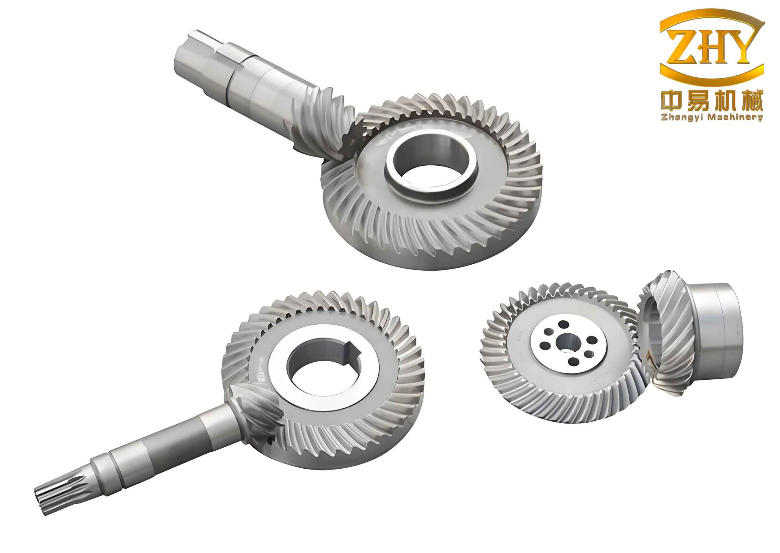
The Geometric Intricacy of the Hyperboloid Gear
The fundamental challenge in modeling a hyperboloid gear lies in its generation process. Unlike parallel axis gears, the tooth surfaces are not simple geometrical shapes but are defined by the complex relative motion between the cutting tool and the gear blank. For the Cyclo-Palloid system, a double-bladed cutter head (one for the convex side, one for the concave side) rotates while a imaginary generating gear, or “crown wheel,” rolls with the workpiece. The tooth profile is a result of the tool’s cutting edge sweeping through this coordinated motion. A complete model must account for every parameter: the cutter geometry (including its nominal radius, blade angles, and tip fillet), its spatial orientation on the machine (tilt, swivel), and the kinematic relationship between the cutter rotation, the generating gear’s rotation, and the workpiece’s rotation. Omitting any element, such as the fillet generated by the tool tip, leads to an incomplete model unsuitable for subsequent stress and durability analysis.
Foundations of Mathematical Modeling: From Cutter Edge to Finished Tooth
My modeling approach begins at the most fundamental level: the cutting edge. We define a coordinate system \( S_t(x_t, y_t, z_t) \) rigidly attached to the rotating cutter head. The straight-line cutting edge of a blade for the convex side of a pinion can be described in its local coordinate system \( S_l(x_l, y_l, z_l) \) by a simple vector function of parameter \( u \):
$$ \mathbf{r}_l(u) = [u \sin(\alpha_0), 0, u \cos(\alpha_0)]^T $$
where \( \alpha_0 \) is the tool blade pressure angle. The crucial fillet surface, generated by the tool tip radius \( r_e \), is defined by another parameter \( \theta \):
$$
\mathbf{r}_l(\theta) = \begin{bmatrix}
(h – r_e(1 – \sin\alpha_0))\tan\alpha_0 \\
0 \\
h – r_e(1 – \sin\alpha_0)
\end{bmatrix} + r_e \begin{bmatrix}
\cos\alpha_0 – \cos(\theta + \alpha_0) \\
0 \\
\sin(\theta + \alpha_0) – \sin\alpha_0
\end{bmatrix}
$$
Through a series of coordinate transformations that incorporate the tool’s eccentric mounting \( (E_{xZ}, \phi_e) \) and its orientation angles \( (\delta_0, \beta_i) \), we map this edge to the cutter head coordinate system: \( \mathbf{r}_t(u) = \mathbf{M}_{tl} \mathbf{r}_l(u) \), where \( \mathbf{M}_{tl} \) is the composite transformation matrix.
The next step involves the generating motion. The cutter head is mounted on a virtual crown wheel. As the cutter rotates by an angle \( \beta \), the crown wheel rotates by a proportional angle \( \phi_{c1} = (z_0 / z_p) \beta \), where \( z_0 \) is the number of cutter blade groups and \( z_p \) is the number of teeth on the virtual crown wheel. Applying this kinematic relationship and the corresponding transformation \( \mathbf{M}_{ct}(\beta) \), we obtain the surface swept by the cutting edge in the crown wheel coordinate system \( S_c \):
$$ \mathbf{r}_c(u, \beta) = \mathbf{M}_{ct}(\beta) \mathbf{r}_t(u) $$
Finally, to generate the actual gear tooth, this crown wheel must roll without slipping against the gear blank. This introduces the fundamental gear generation relationship. If the gear blank rotates by an angle \( \phi_1 \), the crown wheel must rotate by \( \phi_{c2} = (z / z_p) \phi_1 \), where \( z \) is the number of teeth on the actual gear being cut. Applying the final transformation \( \mathbf{M}_{1c}(\phi_1) \), which includes the machine settings like offset, sliding base, and root angle, yields the family of surfaces that define the tooth flank:
$$ \mathbf{r}_1(u, \beta, \phi_1) = \mathbf{M}_{1c}(\phi_1) \mathbf{r}_c(u, \beta) $$
This is not yet a single surface but a family parameterized by \( \phi_1 \). The definitive tooth surface is the envelope of this family, found by imposing the condition of tangency, also known as the equation of meshing:
$$ f_1(u, \beta, \phi_1) = \mathbf{n}_1 \cdot \mathbf{v}_1^{(m1)} = \mathbf{n}_1 \cdot \left( \frac{\partial \mathbf{r}_1}{\partial \phi_1} \right) = 0 $$
Here, \( \mathbf{n}_1 \) is the normal to the family of surfaces, and \( \mathbf{v}_1^{(m1)} \) is the relative velocity between the cutter and the workpiece. Solving the system \( \mathbf{r}_1(u, \beta, \phi_1) \) and \( f_1(u, \beta, \phi_1)=0 \) gives the explicit definition of the pinion’s convex active tooth surface. An identical procedure, with appropriate changes to tool geometry and machine settings, generates the concave side of the gear and the pinion’s concave/gear’s convex sides. This comprehensive model produces the complete, manufacturable tooth geometry, including the vital root fillet. The core parameters defining a typical hyperboloid gear pair are summarized below:
| Parameter | Gear (Concave Side) | Pinion (Convex Side) |
|---|---|---|
| Shaft Angle | 90° | |
| Offset Distance | 40 mm | |
| Normal Module at Ref. Point | 6.065 mm | |
| Number of Teeth | 49 | 12 |
| Spiral Angle at Ref. Point | 42.922° | 30.0° |
| Face Width | 60 mm | 65 mm |
Advanced Tooth Contact Analysis: Beyond Basic Alignment
With accurate mathematical models for both the pinion and gear tooth surfaces, the next critical phase is simulating their meshing under load-free conditions, known as Tooth Contact Analysis (TCA). The traditional TCA approach solves for the contact point by requiring positional and normal vector continuity between the two surfaces in a fixed assembly coordinate system \( S_s \):
$$ \mathbf{r}_s^{(1)}(\phi_1, u_1, \beta_1) = \mathbf{r}_s^{(2)}(\phi_2, u_2, \beta_2) $$
$$ \mathbf{n}_s^{(1)}(\phi_1, u_1, \beta_1) = \mathbf{n}_s^{(2)}(\phi_2, u_2, \beta_2) $$
However, since the normal vectors are unit vectors \( (|\mathbf{n}_s^{(1)}| = |\mathbf{n}_s^{(2)}| = 1) \), the second vector equation provides only two independent scalar equations. This under-constrained system can lead to geometrically incorrect solutions or convergence issues. In my work, I adopt a more robust formulation. Instead of directly equating normals, I enforce that the normal vector of one surface lies within the tangent plane of the mating surface. This is achieved using two orthogonal vectors within that tangent plane. For instance, using the gear’s tangent plane vectors \( (\mathbf{n}_s^{(2)} \times \mathbf{t}_s^{(2)}) \) and \( \mathbf{t}_s^{(2)} \), the contact condition becomes:
$$
\begin{cases}
\mathbf{r}_s^{(1)} – \mathbf{r}_s^{(2)} = 0 \\
(\mathbf{n}_s^{(2)} \times \mathbf{t}_s^{(2)}) \cdot \mathbf{n}_s^{(1)} = 0 \\
\mathbf{t}_s^{(2)} \cdot \mathbf{n}_s^{(1)} = 0
\end{cases}
$$
This system, combined with the two equations of meshing \( f_1=0 \) and \( f_2=0 \) from the generation of each surface, forms a well-constrained set of five independent equations. By taking the pinion rotation angle \( \phi_1 \) as input, we can solve for the remaining five unknowns \( (u_1, \beta_1, u_2, \beta_2, \phi_2) \). The sequence of contact points across the face width forms the path of contact, and the deviation of the output motion from the ideal constant ratio defines the transmission error (TE), a key excitation source for gear noise:
$$ \Delta \phi_2 = (\phi_2 – \phi_{20}) – \frac{z_1}{z_2} (\phi_1 – \phi_{10}) $$
A critical output of TCA is the prediction of the instantaneous contact ellipse, which represents the area of contact under a small applied load due to elastic deformation. Classical methods rely on computing the principal curvatures and directions of both surfaces at the contact point, followed by a complex derivation of the relative curvature. This process is not only cumbersome but also relies on second-order surface approximations that may not accurately reflect the true contact area over larger deformations.
I propose a more direct and accurate iterative method. The concept is to directly probe the separation between the two tooth surfaces around the theoretical contact point. Given a prescribed deformation \( \delta \) (e.g., 0.00635 mm for hardened gears), the contact boundary is the set of points where the separation between the surfaces equals \( \delta \).
- Consider a plane \( Q \) that contains the common surface normal \( \mathbf{u}_3 \) at the contact point.
- Within this plane, find the two points (one on each side along a direction within \( Q \)) where the separation between the two mathematical surfaces \( \Sigma_1 \) and \( \Sigma_2 \) equals \( \delta \). The distance between these two points is a chord \( c \) of the contact ellipse.
- Rotate the plane \( Q \) around the normal axis \( \mathbf{u}_3 \) in small angular steps over 180 degrees. For each orientation, repeat step 2 to find the chord length \( c(\psi) \).
The envelope of all these chords defines the complete contact ellipse boundary. The major axis length is simply \( \max(c(\psi)) \), and its direction is given by the orientation \( \psi \) at which this maximum occurs. This method bypasses complex curvature calculations and works directly with the true hyperboloid gear surface geometry, providing a more reliable prediction of contact pattern size and orientation.
Practical Implementation and Validation
Implementing the models described above requires careful coding of the coordinate transformations and robust numerical solvers. The machine settings for generating a Klingelnberg hyperboloid gear pair are extensive. Below is a subset of critical machine setup parameters for the example gear pair, which directly influence the final tooth geometry and contact pattern.
| Machine Setting Parameter | Gear | Pinion |
|---|---|---|
| Cutter Radial Setting (mm) | 172.038 | 172.038 |
| Initial Cradle Angle (°) | -44.061 | 56.983 |
| Vertical Work Offset (mm) | 4.115 | 35.697 |
| Machine Root Angle (°) | 71.354 | 18.206 |
| Blade Group Count, \(z_0\) | 5 | |
| Virtual Crown Wheel Teeth, \(z_p\) | 50.033 | |
Similarly, the cutter geometry for each side must be precisely defined. The double-blade setup for Klingelnberg cutters involves distinct parameters for the inside and outside blades.
| Cutter Parameter | Gear Concave / Pinion Convex Blade | Gear Convex / Pinion Concave Blade |
|---|---|---|
| Nominal Radius (mm) | 135.461 / 135.397 | 135.0 |
| Blade Pressure Angle (°) | -21 / -19 | 19 / 21 |
| Blade Direction Angle (°) | 6.427 / -6.430 | 6.449 / -6.449 |
| Eccentricity \(E_{xZ}\) (mm) | 3.311 / 3.872 | 0 |
Using these parameters within my modeling and TCA program yields definitive results. The simulated contact pattern for the gear pair shows a well-centered path of contact with a slight bias towards the toe and heel, which is typical and desirable for managing misalignment. The associated transmission error curve is parabolic and low in amplitude, indicating stable and quiet meshing characteristics. These digital results have been validated against physical roll test images of the manufactured gear pair, showing excellent agreement in contact pattern location, shape, and size. This successful validation confirms that the mathematical model accurately represents the physical manufacturing process and that the improved TCA algorithm reliably predicts the gear pair’s functional performance.
Engineering Significance and Future Pathways
The ability to generate a complete digital model of a Klingelnberg Cyclo-Palloid hyperboloid gear and perform high-fidelity TCA is a cornerstone of modern gear design. This virtual prototyping capability allows for the optimization of machine settings and tool geometry to achieve desired contact patterns and low transmission error before any metal is cut, saving significant time and cost. The inclusion of the root fillet surface is essential as it forms the foundation for subsequent Loaded Tooth Contact Analysis (LTCA) and finite element analysis (FEA) for bending stress and root durability calculations.
The improved TCA methodology, with its robust formulation for solving the contact condition and its direct method for computing the contact ellipse, provides more reliable and geometrically accurate results. It eliminates dependencies on approximate curvature calculations and potential numerical instabilities. This framework is not limited to Klingelnberg hyperboloid gears but can be extended and adapted to other gear types with complex generation processes, such as face-milled spiral bevel gears or even worm gears.
Looking forward, the logical next step is the integration of this unloaded TCA model into a full LTCA simulation. This involves iteratively solving for the deformed contact pattern under operational loads, accounting for the stiffness of the teeth, shafts, and bearings. Furthermore, coupling this precise geometry with multi-body dynamic simulation software will enable the prediction of system-level vibrations and noise, closing the loop between design, manufacturing, and performance for the advanced hyperboloid gear drives that power our most demanding mechanical systems.