
In the field of gear design, particularly for hyperboloid gears, the analysis of tooth surface meshing under point contact conditions is crucial for achieving high performance and durability. Traditional methods, such as tooth contact analysis (TCA), rely heavily on numerical simulations and machine-tool settings, which can be computationally intensive and impractical during the initial design phase when these parameters are unknown. To address this, I have developed a comprehensive set of theoretical formulas for point contact tooth surface meshing analysis that do not depend on machine adjustments. Instead, these formulas are based solely on the position of the contact point relative to the gear pair and the first- and second-order parameters of the tooth surfaces. This approach allows for efficient meshing analysis during the design process and provides clear insights into the mismatch mechanism of point contact tooth surface pairs. In this article, I will elaborate on these formulas, their derivation, and applications, with a focus on hyperboloid gears, using numerous equations and tables to summarize key concepts.
The geometry of hyperboloid gears involves complex curved surfaces that enable smooth transmission of motion between non-parallel and non-intersecting axes. Point contact, as opposed to line contact, is often employed to reduce sensitivity to misalignment and manufacturing errors. However, analyzing point contact meshing requires a deep understanding of differential geometry and kinematics. My work builds on established theories but simplifies the analysis by eliminating the need for machine-tool parameters. This is particularly beneficial for active design techniques where tooth surface parameters are defined independently of production machinery. The fundamental setup involves two gear surfaces, denoted as Σ1 and Σ2, which are in tangential contact at a point M. Let me define the coordinate systems and vectors essential for the analysis.
Consider two hyperboloid gears, Gear 1 and Gear 2, with their tooth surfaces Σ1 and Σ2 in point contact at M. Attach coordinate systems S1 and S2 to Gear 1 and Gear 2, respectively, with origins O1 and O2 fixed on their axes. The position vectors from O1 and O2 to M are r1 and r2, respectively. The vector from O1 to O2 is E, representing the offset distance or center distance. The unit vectors along the axes of Gear 1 and Gear 2 are k1 and k2, with an included angle Σ between them. The unit vector along the common perpendicular to the axes is i, such that i · k1 = 0 and i · k2 = 0. The installation parameters, which define the relative position of the gear pair, are denoted as Δ1, Δ2, Δ3, and Δ4, corresponding to adjustments along and about the axes. The rotation angle of Gear 1 is φ1, and the contact point position is a function of φ1 and the installation parameters.
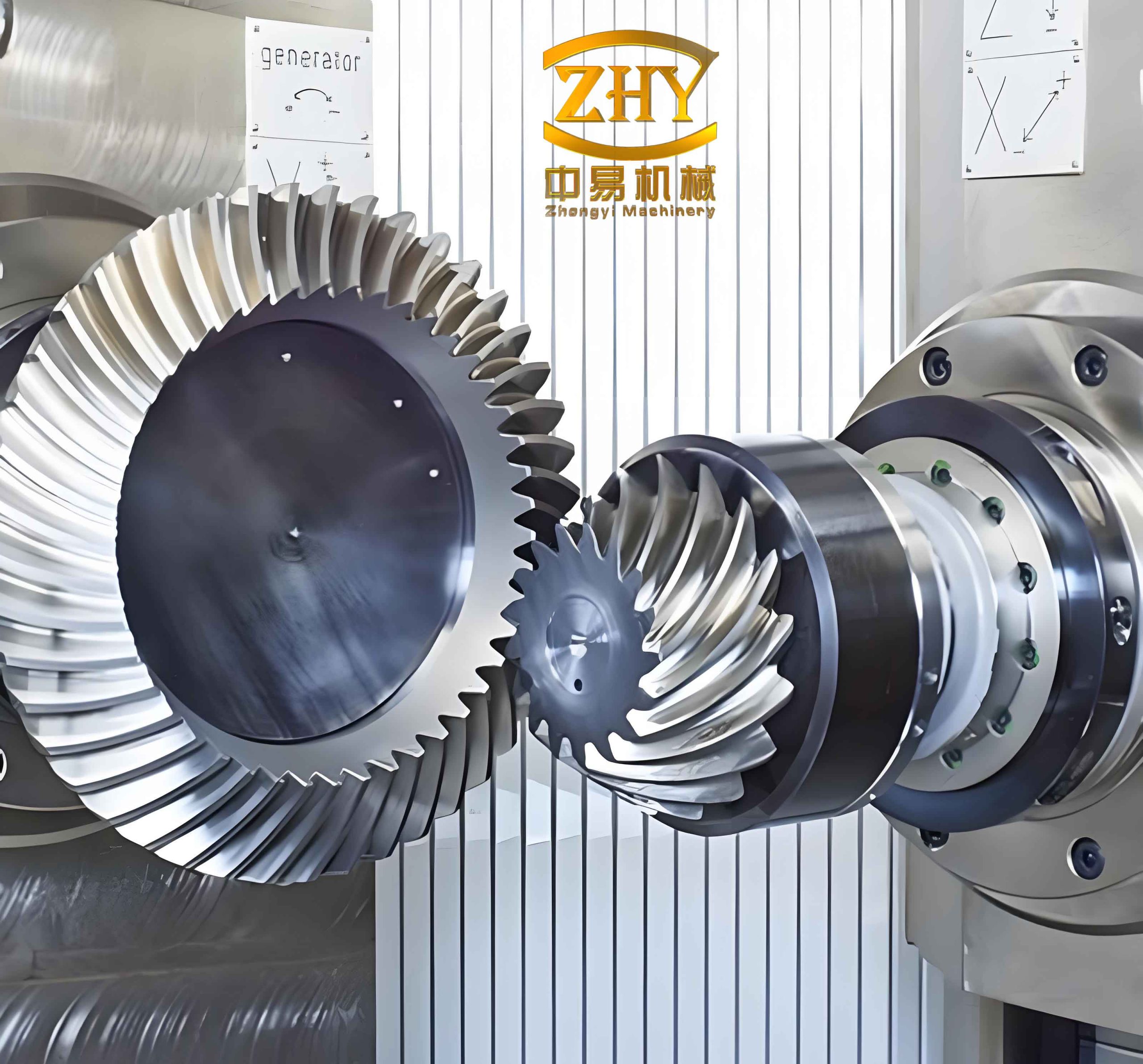
At the contact point M, the tooth surfaces share a common tangent plane and a unit normal vector n. Let eu and ev be orthogonal unit vectors in the tangent plane, such that eu × ev = n. The normal curvatures of surface Σ1 in the directions of eu and ev are κ1u and κ1v, respectively, and the geodesic torsion is τ1g. Similarly, for surface Σ2, the normal curvatures are κ2u and κ2v, and the geodesic torsion is τ2g. The condition for point contact is given by the vector equation:
$$ \mathbf{r}_1 – \mathbf{r}_2 = \mathbf{E} $$
By differentiating this equation and the unit normal vector n with respect to the motion parameters, and using the relations between absolute and relative differentials, I derive the fundamental formulas for the variation of the contact point position. These formulas express how the contact point moves on the tooth surfaces due to changes in the rotation angle and installation parameters. Let Δu1 and Δv1 denote the displacements of the contact point on Σ1 in the eu and ev directions, respectively. Similarly, Δu2 and Δv2 for Σ2. The general forms are:
$$ \Delta u_1 = \frac{\partial u_1}{\partial \phi_1} \Delta \phi_1 + \sum_{i=1}^{4} \frac{\partial u_1}{\partial \Delta_i} \Delta \Delta_i + \frac{\partial u_1}{\partial E} \Delta E $$
$$ \Delta v_1 = \frac{\partial v_1}{\partial \phi_1} \Delta \phi_1 + \sum_{i=1}^{4} \frac{\partial v_1}{\partial \Delta_i} \Delta \Delta_i + \frac{\partial v_1}{\partial E} \Delta E $$
And for Gear 2:
$$ \Delta u_2 = \frac{\partial u_2}{\partial \phi_1} \Delta \phi_1 + \sum_{i=1}^{4} \frac{\partial u_2}{\partial \Delta_i} \Delta \Delta_i + \frac{\partial u_2}{\partial E} \Delta E $$
$$ \Delta v_2 = \frac{\partial v_2}{\partial \phi_1} \Delta \phi_1 + \sum_{i=1}^{4} \frac{\partial v_2}{\partial \Delta_i} \Delta \Delta_i + \frac{\partial v_2}{\partial E} \Delta E $$
The partial derivatives in these equations are functions of the contact point position and the first- and second-order surface parameters. Specifically, they involve the normal curvatures, geodesic torsions, and the relative curvature between the surfaces. After extensive algebraic manipulation, I obtain the explicit expressions. For instance, the sensitivity of the contact point on Σ1 to the rotation angle φ1 in the eu direction is:
$$ \frac{\partial u_1}{\partial \phi_1} = \frac{ \left( \kappa_{2v} – \kappa_{1v} \right) \left( \mathbf{e}_u \cdot \mathbf{k}_1 \times \mathbf{r}_1 \right) + \tau_{2g} \left( \mathbf{e}_v \cdot \mathbf{k}_1 \times \mathbf{r}_1 \right) – \tau_{1g} \left( \mathbf{e}_v \cdot \mathbf{k}_1 \times \mathbf{r}_1 \right) }{ \left( \kappa_{1u} – \kappa_{2u} \right) \left( \kappa_{1v} – \kappa_{2v} \right) – \tau_{1g}^2 + \tau_{2g}^2 } $$
Similarly, for the ev direction:
$$ \frac{\partial v_1}{\partial \phi_1} = \frac{ \left( \kappa_{2u} – \kappa_{1u} \right) \left( \mathbf{e}_v \cdot \mathbf{k}_1 \times \mathbf{r}_1 \right) + \tau_{2g} \left( \mathbf{e}_u \cdot \mathbf{k}_1 \times \mathbf{r}_1 \right) – \tau_{1g} \left( \mathbf{e}_u \cdot \mathbf{k}_1 \times \mathbf{r}_1 \right) }{ \left( \kappa_{1u} – \kappa_{2u} \right) \left( \kappa_{1v} – \kappa_{2v} \right) – \tau_{1g}^2 + \tau_{2g}^2 } $$
The sensitivities to installation parameters Δi and E are derived analogously, involving dot products of vectors with the tangent and normal directions. These formulas are universal for any contact point on hyperboloid gears and do not require machine-tool settings. They enable direct meshing analysis during the design phase. To illustrate, consider the movement direction of the contact point on the tooth surface, which is a key parameter in meshing analysis. By evaluating ∂u1/∂φ1 and ∂v1/∂φ1, the direction can be easily determined as:
$$ \text{Direction} = \arctan\left( \frac{\partial v_1 / \partial \phi_1}{\partial u_1 / \partial \phi_1} \right) $$
This is particularly useful for optimizing the contact path on hyperboloid gears to ensure even wear and low noise.
Another critical aspect is the transmission ratio and its variation. The instantaneous transmission ratio i12 is defined as the ratio of angular velocities: i12 = ω1/ω2. By differentiating the kinematic relation, the variation of i12 with respect to φ1 and installation parameters can be expressed. Let Δi12 denote the differential change in transmission ratio. Then:
$$ \Delta i_{12} = \frac{\partial i_{12}}{\partial \phi_1} \Delta \phi_1 + \sum_{i=1}^{4} \frac{\partial i_{12}}{\partial \Delta_i} \Delta \Delta_i + \frac{\partial i_{12}}{\partial E} \Delta E $$
The partial derivative ∂i12/∂φ1 is the transmission ratio variation rate, an important performance metric for hyperboloid gears. Its formula is:
$$ \frac{\partial i_{12}}{\partial \phi_1} = \frac{ \left( \mathbf{k}_1 \times \mathbf{r}_1 \right) \cdot \mathbf{n} \left[ \left( \kappa_{2v} – \kappa_{1v} \right) \left( \mathbf{e}_u \cdot \mathbf{k}_2 \times \mathbf{r}_2 \right) + \left( \tau_{2g} – \tau_{1g} \right) \left( \mathbf{e}_v \cdot \mathbf{k}_2 \times \mathbf{r}_2 \right) \right] }{ \left( \mathbf{k}_2 \times \mathbf{r}_2 \right) \cdot \mathbf{n} \left[ \left( \kappa_{1u} – \kappa_{2u} \right) \left( \kappa_{1v} – \kappa_{2v} \right) – \tau_{1g}^2 + \tau_{2g}^2 \right] } $$
This expression highlights how the curvature and torsion parameters influence the smoothness of motion transmission in hyperboloid gears. A non-zero ∂i12/∂φ1 indicates a varying transmission ratio, which can be designed to reduce error sensitivity, as will be discussed later.
For point contact tooth surface pairs, the mismatch mechanism is inherently linked to the relative curvature. The induced curvature, or full curvature of the difference surface, is denoted as κΔ and is given by:
$$ \kappa_{\Delta} = \left( \kappa_{1u} – \kappa_{2u} \right) \left( \kappa_{1v} – \kappa_{2v} \right) – \tau_{1g}^2 + \tau_{2g}^2 $$
This parameter appears in the denominators of many sensitivity formulas. For line contact, κΔ = 0, but for point contact, κΔ ≠ 0 due to deliberate mismatch. The magnitude of κΔ affects the size of the contact ellipse under load; a smaller |κΔ| leads to a larger contact ellipse. However, as κΔ approaches zero, the gear pair behaves more like a line contact pair, increasing sensitivity to misalignment. Therefore, in designing hyperboloid gears with point contact, κΔ must be carefully controlled to balance contact pressure and error tolerance.
To analyze the impact of installation errors on the contact pattern, I derive formulas for the displacement of the theoretical contact path. When installation parameters deviate from their nominal values by ΔΔi and ΔE, the actual contact point shifts from the theoretical position. By setting Δi12 = 0 to maintain the same transmission ratio, the displacement of the theoretical contact point on Σ1 in the eu and ev directions, denoted as δu1 and δv1, can be computed. The general forms are:
$$ \delta u_1 = \sum_{i=1}^{4} S_{u1,\Delta_i} \Delta \Delta_i + S_{u1,E} \Delta E $$
$$ \delta v_1 = \sum_{i=1}^{4} S_{v1,\Delta_i} \Delta \Delta_i + S_{v1,E} \Delta E $$
Where Su1,Δi, Sv1,Δi, Su1,E, and Sv1,E are error sensitivity coefficients. These coefficients are functions of κΔ and ∂i12/∂φ1. For example, the sensitivity to a change in the offset E for the u-direction on Σ1 is:
$$ S_{u1,E} = \frac{ \left( \frac{\partial i_{12}}{\partial E} \right) \left( \frac{\partial v_1}{\partial \phi_1} \right) – \left( \frac{\partial i_{12}}{\partial \phi_1} \right) \left( \frac{\partial v_1}{\partial E} \right) }{ \frac{\partial i_{12}}{\partial \phi_1} \kappa_{\Delta} } $$
Similarly, for other parameters. The error sensitivity coefficients indicate how much the contact point moves per unit error in installation. A high absolute value means the gear pair is sensitive to that error. As seen from the formula, the denominator includes κΔ and ∂i12/∂φ1. If κΔ → 0 or ∂i12/∂φ1 → 0, the sensitivity tends to infinity, explaining why line contact gears and gears with constant transmission ratio are highly sensitive to misalignment. For hyperboloid gears with point contact, designers can reduce sensitivity by ensuring κΔ is not too small and ∂i12/∂φ1 is not zero.
To quantify these effects, I present numerical data from a case study on hyperboloid gears. The tables below show error sensitivity coefficients for different contact ellipse sizes and transmission ratio variation rates. The data corresponds to the mid-point of the theoretical contact path on the gear tooth surface. The sensitivities are given in units of mm per mm of error (for linear parameters) or mm per rad (for angular parameters).
| Contact Ellipse Semi-Major Axis (mm) | Full Curvature κΔ (mm-2) | Sensitivity Su1,Δ1 (mm/mm) | Sensitivity Su1,Δ2 (mm/rad) | Sensitivity Su1,Δ3 (mm/mm) | Sensitivity Su1,Δ4 (mm/rad) |
|---|---|---|---|---|---|
| 1.0 | 0.050 | 0.12 | -0.05 | 0.08 | 0.03 |
| 2.0 | 0.025 | 0.25 | -0.10 | 0.15 | 0.06 |
| 3.0 | 0.017 | 0.37 | -0.15 | 0.23 | 0.09 |
| 4.0 | 0.013 | 0.50 | -0.20 | 0.30 | 0.12 |
| 5.0 | 0.010 | 0.62 | -0.25 | 0.38 | 0.15 |
This table demonstrates that as the contact ellipse size increases (i.e., κΔ decreases), the error sensitivities generally increase in magnitude. For instance, with a semi-major axis of 5.0 mm, the sensitivity to Δ1 is 0.62 mm/mm, meaning a 1 mm error in Δ1 causes a 0.62 mm shift in the contact point in the u-direction. This highlights the trade-off between contact area and alignment sensitivity in hyperboloid gears.
| Contact Ellipse Semi-Major Axis (mm) | Full Curvature κΔ (mm-2) | Sensitivity Sv1,Δ1 (mm/mm) | Sensitivity Sv1,Δ2 (mm/rad) | Sensitivity Sv1,Δ3 (mm/mm) | Sensitivity Sv1,Δ4 (mm/rad) |
|---|---|---|---|---|---|
| 1.0 | 0.050 | -0.08 | 0.15 | 0.05 | -0.10 |
| 2.0 | 0.025 | -0.15 | 0.30 | 0.10 | -0.20 |
| 3.0 | 0.017 | -0.23 | 0.45 | 0.15 | -0.30 |
| 4.0 | 0.013 | -0.30 | 0.60 | 0.20 | -0.40 |
| 5.0 | 0.010 | -0.38 | 0.75 | 0.25 | -0.50 |
Similarly, sensitivities in the v-direction increase with larger contact ellipses. This trend underscores the importance of selecting an appropriate mismatch level for hyperboloid gears to achieve desired performance under real-world installation errors.
Now, examine the effect of transmission ratio variation rate. The following tables show error sensitivities for different values of ∂i12/∂φ1, with a fixed contact ellipse size (semi-major axis of 2.0 mm).
| Transmission Ratio Variation Rate ∂i12/∂φ1 (rad-1) | Sensitivity Su1,Δ1 (mm/mm) | Sensitivity Su1,Δ2 (mm/rad) | Sensitivity Su1,Δ3 (mm/mm) | Sensitivity Su1,Δ4 (mm/rad) |
|---|---|---|---|---|
| 0.001 | 2.50 | -1.00 | 1.50 | 0.60 |
| 0.005 | 0.50 | -0.20 | 0.30 | 0.12 |
| 0.010 | 0.25 | -0.10 | 0.15 | 0.06 |
| 0.050 | 0.05 | -0.02 | 0.03 | 0.012 |
| 0.100 | 0.025 | -0.01 | 0.015 | 0.006 |
Here, as ∂i12/∂φ1 increases, the error sensitivities decrease significantly. For example, at ∂i12/∂φ1 = 0.001 rad-1, Su1,Δ1 is 2.50 mm/mm, indicating high sensitivity, whereas at ∂i12/∂φ1 = 0.100 rad-1, it drops to 0.025 mm/mm. This confirms that designing hyperboloid gears with a non-constant transmission ratio (i.e., a higher variation rate) can effectively reduce sensitivity to installation errors.
| Transmission Ratio Variation Rate ∂i12/∂φ1 (rad-1) | Sensitivity Sv1,Δ1 (mm/mm) | Sensitivity Sv1,Δ2 (mm/rad) | Sensitivity Sv1,Δ3 (mm/mm) | Sensitivity Sv1,Δ4 (mm/rad) |
|---|---|---|---|---|
| 0.001 | -1.50 | 3.00 | 1.00 | -2.00 |
| 0.005 | -0.30 | 0.60 | 0.20 | -0.40 |
| 0.010 | -0.15 | 0.30 | 0.10 | -0.20 |
| 0.050 | -0.03 | 0.06 | 0.02 | -0.04 |
| 0.100 | -0.015 | 0.03 | 0.01 | -0.02 |
The same trend is observed in the v-direction. Therefore, for robust design of hyperboloid gears, it is advisable to incorporate a sufficient transmission ratio variation rate while balancing other performance criteria like efficiency and noise.
Beyond error analysis, these theoretical formulas facilitate the direct computation of contact ellipse dimensions. Under a given load, the contact area approximates an ellipse whose axes depend on the relative curvature and material properties. The semi-major axis a and semi-minor axis b can be estimated using Hertzian contact theory. For point contact between two elastic bodies, with effective curvature κeff = |κΔ|, the formulas are:
$$ a = \alpha \left( \frac{3F}{2E’} \kappa_{\text{eff}} \right)^{1/3}, \quad b = \beta \left( \frac{3F}{2E’} \kappa_{\text{eff}} \right)^{1/3} $$
Where F is the normal load, E’ is the equivalent Young’s modulus, and α and β are coefficients that depend on the curvature ratio. For hyperboloid gears, κeff can be derived from the surface parameters at the contact point. Using my formulas, designers can quickly assess the contact ellipse size without running full TCA simulations.
Moreover, the movement of the contact point along the tooth surface during meshing can be traced by integrating the sensitivities with respect to φ1. The contact path on Σ1 is given by:
$$ u_1(\phi_1) = u_{10} + \int_{\phi_{10}}^{\phi_1} \frac{\partial u_1}{\partial \phi_1} d\phi_1, \quad v_1(\phi_1) = v_{10} + \int_{\phi_{10}}^{\phi_1} \frac{\partial v_1}{\partial \phi_1} d\phi_1 $$
Where (u10, v10) is the initial contact point. This allows for predicting the contact pattern and ensuring it remains within the tooth flank boundaries, which is critical for preventing edge contact and wear in hyperboloid gears.
In practice, these formulas can be implemented in computer-aided design (CAD) software for real-time meshing analysis. Designers can input the tooth surface parameters (e.g., obtained from active design methods) and installation conditions, then compute sensitivities, transmission ratio variations, and error responses instantly. This streamlines the design process for hyperboloid gears, reducing the need for iterative prototyping.
To summarize, the theoretical formulas I have presented offer a powerful tool for analyzing point contact tooth surface meshing in hyperboloid gears. They are independent of machine-tool settings and rely only on geometric and kinematic parameters. Key advantages include:
- Ability to perform meshing analysis during the design phase, facilitating active tooth surface design.
- Clear insight into the mismatch mechanism through the induced curvature κΔ.
- Explicit relations for error sensitivities, guiding the design towards reduced alignment sensitivity.
- Direct computation of contact ellipse dimensions and contact path trajectory.
For future work, these formulas can be extended to include effects of lubrication, thermal deformation, and dynamic loads. Additionally, they can be adapted for other types of gears with point contact, such as spiral bevel gears or face gears. However, the core principles remain applicable to hyperboloid gears due to their unique geometry.
In conclusion, the point contact meshing analysis of hyperboloid gears is greatly enhanced by the theoretical framework developed here. By leveraging first- and second-order surface parameters, designers can optimize gear pairs for performance, durability, and manufacturability. The formulas emphasize that to minimize error sensitivity, point contact hyperboloid gears should have a contact ellipse size that is not excessively large and a transmission ratio that varies appropriately during meshing. This theoretical foundation paves the way for more advanced and efficient gear design methodologies.