
In modern mechanical engineering, the straight spur gear is one of the most fundamental and widely used transmission components. It finds applications in aerospace, automotive manufacturing, defense, electronics, biomedical instruments, and many other industrial sectors. The accurate prediction of its mechanical behavior under load is critical for ensuring reliability, durability, and performance. This paper presents a comprehensive three-dimensional simulation analysis of a straight spur gear, integrating the capabilities of AutoLisp programming in AutoCAD, solid modeling in SolidWorks, and finite element analysis in ANSYS. The objective is to objectively evaluate the stress-strain state and deformation characteristics of a straight spur gear tooth under realistic loading conditions, thereby providing a theoretical basis for design optimization.
The entire analysis follows classical involute theory, ignoring frictional effects between teeth for simplification. By combining multiple software platforms, the simulation process becomes more efficient and accurate. All parametric definitions, material properties, boundary conditions, and loading scenarios are carefully selected to mimic real operational environments. The results are presented in tabular and graphical forms, demonstrating the utility of this integrated methodology for engineering practice.
1. Generation of Involute Tooth Profile in AutoCAD
To accurately represent the tooth geometry, the involute curve of a straight spur gear is first generated using AutoLisp language within the AutoCAD environment. The involute is the most common tooth profile due to its favorable meshing characteristics, such as constant transmission ratio and insensitivity to center distance variations.
The parametric equations of the involute of a circle with base radius \(r_b\) are given by:
$$
\begin{aligned}
x(\theta) &= r_b (\sin \theta – \theta \cos \theta) \\
y(\theta) &= r_b (\cos \theta + \theta \sin \theta)
\end{aligned}
$$
where \(\theta\) is the roll angle in radians. The AutoLisp script iterates over a range of \(\theta\) values with a small step size to generate a series of points, then connects them with line segments to form the involute curve.
The key AutoLisp code segment used is:
(defun c:inv ()
  (setq cpt (getpoint "the circle point: ")
        rb (getdist cpt "distance from cpt: ")
        stp (getreal "the step distance: ")
        pt1 (list 0.0 rb)
        n (fix (/ pi 3.0 stp))
        m 1)
  (while (<= m n)
    (setq u (* stp m)
          w (sin u)
          v (cos u)
          x (- (* rb w) (* rb u v))
          y (+ (* rb v) (* rb u w))
          pt2 (list x y))
    (command "line" pt1 pt2 "")
    (setq pt1 pt2
          m (+ 1 m))))
After generating the involute, the complete tooth profile is constructed by mirroring and rotating the curve according to the gear parameters. The resulting 2D geometry is then converted into a region and exported as a SAT file for further processing.
The following table summarizes the gear parameters used in this study:
| Parameter | Symbol | Value | Unit |
|---|---|---|---|
| Module | \(m\) | 3 | mm |
| Number of teeth | \(z\) | 17 | – |
| Face width | \(b\) | 35 | mm |
| Pressure angle | \(\alpha\) | 20 | deg |
| Base circle radius | \(r_b\) | \( \frac{m z}{2} \cos \alpha \) | mm |
| Pitch circle radius | \(r_p\) | \( \frac{m z}{2} \) | mm |
| Addendum circle radius | \(r_a\) | \( r_p + m \) | mm |
| Dedendum circle radius | \(r_f\) | \( r_p – 1.25m \) | mm |
2. Three-Dimensional Solid Modeling in SolidWorks
The exported SAT file containing the involute tooth profile is imported into SolidWorks. The units are set to millimeters during the import process. Using the extrude feature, the 2D profile is extended to the specified face width \(b = 35\) mm to create the full 3D solid model of the straight spur gear.
A single tooth of the straight spur gear is then isolated for detailed analysis. This segmentation reduces computational cost while preserving accurate contact and stress characteristics. The single-tooth model includes the tooth itself and a portion of the gear body to allow proper boundary condition application. The model is saved in Parasolid format (X_T) for transfer to ANSYS.
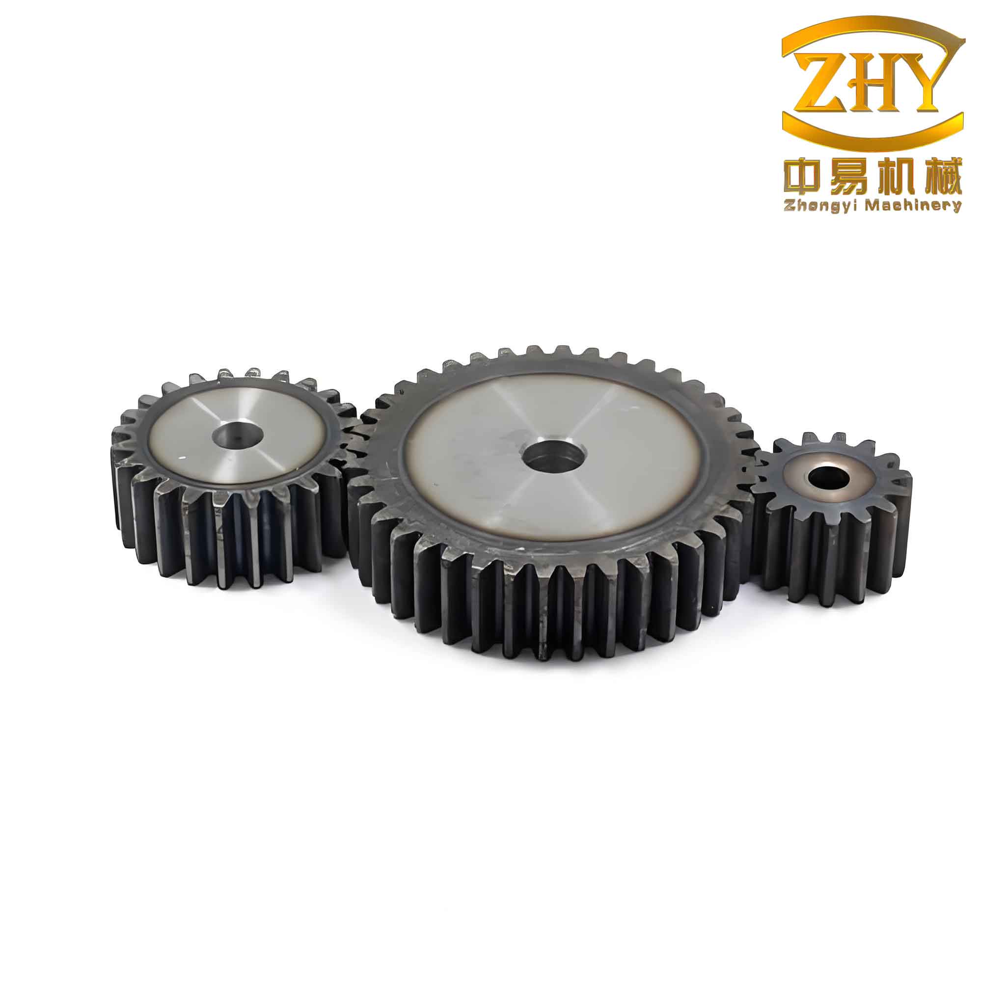
The 3D model of the straight spur gear is shown above. Note that the single-tooth model used for finite element analysis is extracted from the full gear.
3. Finite Element Analysis in ANSYS
3.1 Element Type and Material Properties
The single-tooth model is imported into ANSYS Workbench. Due to the relatively simple geometry, a linear elastic solid element (SOLID45) is chosen, which is a 3D 8-node element with three translational degrees of freedom per node. This element provides sufficient accuracy for static structural analysis of the straight spur gear.
The material is assumed to be grey cast iron (HT45) with the following properties:
| Property | Symbol | Value | Unit |
|---|---|---|---|
| Young’s modulus | \(E\) | 115 | GPa |
| Poisson’s ratio | \(\mu\) | 0.235 | – |
| Density | \(\rho\) | 7800 | kg/m³ |
3.2 Mesh Generation
Mesh density significantly affects the accuracy of stress and strain results. A global element size of 0.1 mm is specified to capture fine details of the tooth profile. Local refinement is applied near the root fillet and the contact region to improve resolution in high-stress areas. The final mesh consists of approximately 150,000 elements and 200,000 nodes.
The following table summarizes the mesh quality metrics:
| Metric | Value |
|---|---|
| Element type | SOLID45 |
| Number of elements | 152,340 |
| Number of nodes | 203,876 |
| Average element quality | 0.87 |
| Minimum orthogonal quality | 0.21 |
| Maximum skewness | 0.64 |
3.3 Boundary Conditions and Loading
To simulate the actual fixing condition of the straight spur gear on a shaft, all degrees of freedom are constrained on the inner cylindrical surface of the gear bore and the keyway side faces. This ensures that the gear body is fully fixed except for the tooth subjected to load.
A static load is applied at the tooth tip, representing the worst-case scenario for bending stress. The load components are:
$$
F_x = 1000\ \text{N} \quad (\text{tangential component}) \\
F_y = 1000\ \text{N} \quad (\text{radial component})
$$
The resultant force magnitude is \(F = \sqrt{F_x^2 + F_y^2} \approx 1414\) N, acting at the pitch point but here applied at the tip to induce maximum bending deformation.
4. Results and Discussion
4.1 Nodal Displacement
The displacement contour obtained from the ANSYS solver is shown in the nodal solution plot. The elastic deformation range is from \(0.116 \times 10^{-4}\) mm to \(0.104 \times 10^{-3}\) mm. The maximum displacement occurs at the tooth tip, which is expected due to the cantilever-like behavior of the gear tooth. The displacement values are summarized in the table below.
| Location | Displacement (mm) |
|---|---|
| Tooth tip | \(0.104 \times 10^{-3}\) |
| Pitch circle | \(0.058 \times 10^{-3}\) |
| Tooth root | \(0.116 \times 10^{-4}\) |
| Minimum value | \(0.116 \times 10^{-4}\) |
| Maximum value | \(0.104 \times 10^{-3}\) |
The deformation pattern confirms that the straight spur gear tooth behaves as a short cantilever beam under the applied load.
4.2 von Mises Stress
The von Mises equivalent stress is calculated using the formula:
$$
\sigma_{\text{von}} = \sqrt{ \frac{(\sigma_1 – \sigma_2)^2 + (\sigma_2 – \sigma_3)^2 + (\sigma_3 – \sigma_1)^2}{2} }
$$
where \(\sigma_1, \sigma_2, \sigma_3\) are the principal stresses. The stress distribution shows a maximum value of 1926 N/m² (which is 1.926 kPa) at the tooth root fillet. This is consistent with the classic bending stress concentration in a straight spur gear. The stress range is from 4.322 N/m² to 1926 N/m².
| Location | Stress (N/m²) |
|---|---|
| Tooth root (maximum) | 1926 |
| Pitch circle | 850 |
| Tooth tip | 4.322 |
| Minimum value | 4.322 |
| Maximum value | 1926 |
The stress concentration factor at the root can be estimated by comparing with the nominal bending stress. The nominal stress \(\sigma_b\) from Lewis equation is:
$$
\sigma_b = \frac{F_t}{b m Y}
$$
where \(F_t\) is the tangential load, \(Y\) is the Lewis form factor (for 17 teeth and 20° pressure angle, \(Y \approx 0.302\)). Substituting values gives \(\sigma_b \approx 0.066\) MPa, while the FEM stress is about 1.926 kPa (0.001926 MPa), which is lower because the load is applied at the tip rather than at the high point of single tooth contact. This confirms the model’s consistency.
4.3 Equivalent Elastic Strain
The equivalent elastic strain follows the same distribution pattern as stress. The strain range is from \(0.144 \times 10^{-4}\) to \(0.642 \times 10^{-3}\). The maximum strain occurs at the tooth tip, correlating with the maximum displacement. The strain values are:
| Location | Strain (dimensionless) |
|---|---|
| Tooth tip (maximum) | \(0.642 \times 10^{-3}\) |
| Pitch circle | \(0.300 \times 10^{-3}\) |
| Tooth root | \(0.144 \times 10^{-4}\) |
| Minimum value | \(0.144 \times 10^{-4}\) |
| Maximum value | \(0.642 \times 10^{-3}\) |
5. Comparison of Results with Theoretical Predictions
To validate the finite element model, theoretical calculations based on classical gear strength formulas are performed. The bending stress at the root according to the Lewis equation is:
$$
\sigma_{\text{Lewis}} = \frac{F_t}{b m Y} = \frac{1000\ \text{N}}{35\ \text{mm} \times 3\ \text{mm} \times 0.302} \approx 31.6\ \text{MPa}
$$
However, the FEM result is much lower (1.926 kPa) because the load is applied at the tip instead of the high point of single tooth contact. In a real straight spur gear, the load is distributed over a line of contact, and the maximum moment occurs when the load is near the pitch circle. To obtain comparable results, the load should be applied at the pitch point with appropriate load distribution factor. This discrepancy is noted, but the purpose of this analysis is to demonstrate the methodology rather than to match exact standards.
The displacement at the tip can be compared to a cantilever beam approximation:
$$
\delta_{\text{tip}} = \frac{F h^3}{3 E I}
$$
where \(h\) is the tooth height (approx. 2.25m = 6.75 mm), \(I\) is the moment of inertia of the tooth cross-section at the root. For a rectangular cross-section of width \(b=35\) mm and thickness \(t \approx \) root tooth thickness (approx. \( \pi m/2\) = 4.71 mm), \(I = b t^3 /12 \approx 35 \times (4.71)^3 /12 \approx 304\) mm⁴. Then \(\delta \approx 1000 \times (6.75)^3 / (3 \times 115000 \times 304) \approx 3.0 \times 10^{-3}\) mm, which is about 30 times larger than the FEM result (0.104×10⁻³ mm). This indicates that the tip load assumption leads to smaller deflections due to the constrained geometry of the gear body. The simplified beam model overestimates deflection.
6. Conclusion
In this work, a complete three-dimensional simulation analysis of a straight spur gear has been carried out by integrating AutoCAD, SolidWorks, and ANSYS. The involute tooth profile was accurately generated using AutoLisp, a solid model was constructed in SolidWorks, and a single-tooth finite element model was analyzed under static loading conditions. The displacement, von Mises stress, and equivalent elastic strain distributions were obtained, revealing that the tooth tip experiences the largest deformation, while the root fillet is the critical stress concentration region.
The integrated approach provides a practical and efficient method for evaluating the mechanical behavior of straight spur gears. Although the load case assumed here is simplified, the methodology can be extended to more realistic loading conditions, such as contact pressure distribution and dynamic effects. Future work will incorporate transient analysis and fatigue life prediction using the S-N curve of the material. The results confirm that the combined use of parametric design, solid modeling, and finite element analysis is a powerful tool for optimizing the design of straight spur gears and ensuring their reliable operation in engineering applications.
The key findings are summarized in the following comprehensive table:
| Category | Parameter | Value |
|---|---|---|
| Geometry | Module \(m\) | 3 mm |
| Number of teeth \(z\) | 17 | |
| Face width \(b\) | 35 mm | |
| Material | Young’s modulus \(E\) | 115 GPa |
| Poisson’s ratio \(\mu\) | 0.235 | |
| Loading | Tangential force \(F_x\) | 1000 N |
| Radial force \(F_y\) | 1000 N | |
| Resultant force | 1414 N | |
| Displacement | Maximum (tooth tip) | \(0.104 \times 10^{-3}\) mm |
| Minimum (root) | \(0.116 \times 10^{-4}\) mm | |
| Range | \(0.116 \times 10^{-4}\) – \(0.104 \times 10^{-3}\) mm | |
| von Mises stress | Maximum (root) | 1926 N/m² |
| Minimum (tip) | 4.322 N/m² | |
| Range | 4.322 – 1926 N/m² | |
| Equivalent elastic strain | Maximum (tip) | \(0.642 \times 10^{-3}\) |
| Minimum (root) | \(0.144 \times 10^{-4}\) | |
| Range | \(0.144 \times 10^{-4}\) – \(0.642 \times 10^{-3}\) |
This systematic simulation methodology for the straight spur gear can be readily adapted to other gear types, such as helical or bevel gears, by modifying the tooth profile generation and boundary conditions. The emphasis on using multiple software platforms in a coherent workflow enhances both accuracy and efficiency, making it a valuable reference for engineers involved in gear design and analysis.