
Spur gear drives are among the most widely used power transmission components in industrial machinery. Their high efficiency, stable transmission ratio, and compact geometry make them indispensable in aerospace, marine, automotive, and mining applications. Nevertheless, the inherent time-varying mesh stiffness of a spur gear pair is a major source of vibration and noise. In this research, a finite element modeling approach is developed for a two-stage spur gear transmission system under multi-source time-varying excitation. The model simultaneously considers gear time-varying mesh stiffness, bearing time-varying stiffness, transmission errors, shaft flexibility, and the two-stage phase relationship. Using the Newmark time-domain integration method, the dynamic response of the geared rotor-bearing system is obtained. The influence of shafting stiffness, bearing stiffness variation, and assembly position on the dynamic characteristics of the two-stage spur gear system is then thoroughly analyzed.
1. Introduction
The dynamic behavior of gear transmission systems has been studied for several decades. Early investigations were based on lumped-parameter models, where the gear pair was represented by rigid inertias connected through a spring along the line of action. A single-degree-of-freedom model can predict the fundamental torsional response of a gear pair, but it cannot capture the coupled bending-torsion motion of the shaft and bearings. Consequently, more refined models were developed, including gear-rotor-bearing models, coupled multi-body models, and finite element models.
For a two-stage spur gear transmission, the system consists of input, intermediate, and output shafts, together with four gears and six rolling-element bearings. The dynamic interaction between the gear meshes, the flexibility of the shafts, and the time-varying support stiffness of the bearings produces a rich vibration spectrum. A pure torsional model cannot predict bearing loads or bearing vibration. Therefore, a generalized finite element formulation is necessary. In this work, the transmission system is discretized into shaft elements, gear mesh elements, and bearing elements. Each element is formulated separately and then assembled into a global system. The approach is efficient, modular, and can be easily adapted to other parallel-axis spur gear systems.
The main contributions of this research are summarized as follows. First, a finite element model of a two-stage spur gear transmission is established that includes not only gear mesh stiffness variation but also the time-varying stiffness of deep-groove ball bearings. Second, the effect of shaft flexibility and shaft stiffness variation on natural frequencies, mode shapes, resonance speeds, and bearing load distribution is analyzed. Third, the influence of the two-stage phase angle and gear mounting position is studied. Finally, the model is validated by comparison with acceleration measurements on a gear transmission test rig.
2. System Description and Finite Element Discretization
The two-stage spur gear transmission considered here is typical of industrial gear reducers. The active gear of the first stage is located on the input shaft, while the driven gear of the first stage is mounted on the intermediate shaft. The second-stage active gear is also mounted on the intermediate shaft, and the second-stage driven gear is placed on the output shaft. Six deep-groove ball bearings support the three shafts. The basic parameters of the shafts and spur gears are listed in Tables 1 and 2, respectively.
| Parameter | Input shaft | Intermediate shaft | Output shaft |
|---|---|---|---|
| Length (m) | 0.24 | 0.16 | 0.18 |
| Radius (mm) | 12.5 | 12.5 | 12.5 |
| Density (kg/m3) | 7850 | 7850 | 7850 |
| Shear modulus (Pa) | 8×10¹⁰ | 8×10¹⁰ | 8×10¹⁰ |
| Gear | Number of teeth | Module (mm) | Pressure angle (°) | Face width (mm) | Mass (kg) | Moment of inertia (kg·m2) |
|---|---|---|---|---|---|---|
| First-stage pinion | 36 | 1.5 | 20 | 12 | 0.16 | 2×10⁻⁴ |
| First-stage gear | 90 | 1.5 | 20 | 12 | 1.3 | 3.04×10⁻³ |
| Second-stage pinion | 29 | 1.5 | 20 | 12 | 0.09 | 1×10⁻⁴ |
| Second-stage gear | 100 | 1.5 | 20 | 12 | 1.6 | 8.71×10⁻³ |
The continuous gear shaft system is discretized along the shaft axis. The input shaft is divided into twelve elements, the intermediate shaft into eight elements, and the output shaft into nine elements. Thus, the complete two-stage spur gear system comprises 29 shaft elements, two gear mesh elements, and six bearing elements. Each node has three degrees of freedom: two transverse translations and one torsional rotation. The global nodal displacement vector is expressed as
\[
\mathbf{q} = [q_1, q_2, q_3, \ldots, q_{95}]^T
\]
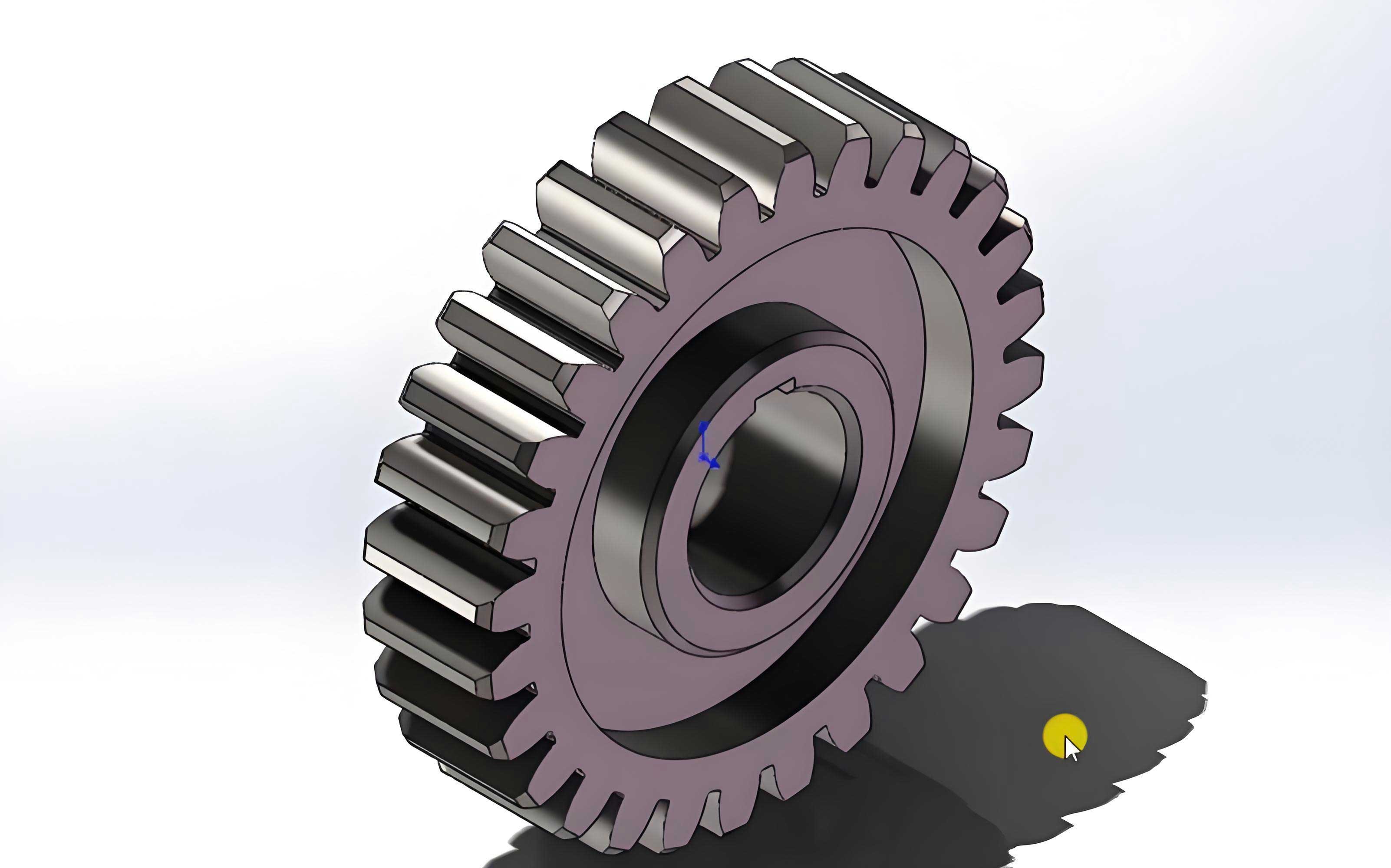
where 95 is the total number of degrees of freedom. The physical arrangement of a spur gear pair used in the modeling is illustrated below.
3. Element Formulations
3.1 Shaft element
Because the diameter-to-length ratio of the shaft is not very small, the shear deformation cannot be ignored. Therefore, the shaft is modeled using the Timoshenko beam theory. For a shaft element of length \(l\), cross-sectional area \(A\), polar moment of inertia \(J\), shear modulus \(G\), and shear correction factor \(\kappa\), the element nodal displacement vector is
\[
\mathbf{q}_s^e = [v_i,\; w_i,\; \theta_i,\; v_j,\; w_j,\; \theta_j]^T
\]
where \(v\) and \(w\) are the two transverse displacements, and \(\theta\) is the torsional rotation. The element stiffness matrix can be written as
\[
\mathbf{K}_s^e =
\begin{bmatrix}
\frac{GA}{\kappa l} & 0 & 0 & -\frac{GA}{\kappa l} & 0 & 0\\
0 & \frac{GA}{\kappa l} & 0 & 0 & -\frac{GA}{\kappa l} & 0\\
0 & 0 & \frac{GJ}{l} & 0 & 0 & -\frac{GJ}{l}\\
-\frac{GA}{\kappa l} & 0 & 0 & \frac{GA}{\kappa l} & 0 & 0\\
0 & -\frac{GA}{\kappa l} & 0 & 0 & \frac{GA}{\kappa l} & 0\\
0 & 0 & -\frac{GJ}{l} & 0 & 0 & \frac{GJ}{l}
\end{bmatrix}
\]
The corresponding consistent mass matrix is
\[
\mathbf{M}_s^e = \frac{\rho A l}{6}
\begin{bmatrix}
2 & 0 & 0 & 1 & 0 & 0\\
0 & 2 & 0 & 0 & 1 & 0\\
0 & 0 & \frac{2J}{A} & 0 & 0 & \frac{J}{A}\\
1 & 0 & 0 & 2 & 0 & 0\\
0 & 1 & 0 & 0 & 2 & 0\\
0 & 0 & \frac{J}{A} & 0 & 0 & \frac{2J}{A}
\end{bmatrix}
\]
Rayleigh damping is used for the shaft element, namely
\[
\mathbf{C}_s^e = \alpha_R \mathbf{M}_s^e + \beta_R \mathbf{K}_s^e
\]
where \(\alpha_R\) and \(\beta_R\) are proportional damping coefficients.
3.2 Gear mesh element
For a spur gear pair, the mesh action is represented by a time-varying spring acting along the line of action. The pinion and gear have translations \(v_p, w_p\) and \(v_g, w_g\) together with torsional rotations \(\theta_p\) and \(\theta_g\). The mesh deflection is the difference between the projections of the pinion and gear displacements in the direction of the line of action. Let \(\alpha\) be the transverse pressure angle and \(r_p, r_g\) the base radii of the pinion and gear. The mesh deflection is
\[
\delta_m = \left(v_p\sin\alpha + w_p\cos\alpha – r_p\theta_p\right) – \left(v_g\sin\alpha + w_g\cos\alpha + r_g\theta_g\right) – e(t)
\]
where \(e(t)\) is the combined transmission error excitation. The elastic mesh force is
\[
F_m = k_m(t)\delta_m
\]
The gear mesh stiffness matrix \(\mathbf{K}_m(t)\) is then
\[
\mathbf{K}_m(t) = k_m(t)\mathbf{u}\mathbf{u}^T
\]
with
\[
\mathbf{u} = [\sin\alpha,\; \cos\alpha,\; -r_p,\; -\sin\alpha,\; -\cos\alpha,\; -r_g]^T
\]
The time-varying mesh stiffness \(k_m(t)\) is obtained from a finite element contact analysis of the spur gear pair. A contact model is solved at several rotational positions within one mesh cycle. The mesh stiffness curve exhibits a periodic variation with the tooth engagement frequency.
3.3 Bearing element
Deep-groove ball bearings are modeled as time-varying stiffness elements. The radial load-deflection relation of a ball bearing is nonlinear and depends on the position of the balls. Considering the alternating arrangement of loaded balls under both odd and even loading conditions, the equivalent bearing stiffness is approximated as a static stiffness plus a periodic fluctuation. The time-dependent bearing stiffness can be expressed as
\[
k_b(t) = k_{bs} + k_a \sin(2\pi f_b t + \beta_b)
\]
where \(k_{bs}\) is the static stiffness, \(k_a\) is the fluctuation amplitude, \(f_b\) is the ball-passing frequency, and \(\beta_b\) is the initial phase. The bearing geometry used in this model is listed in Table 3.
| Parameter | Value |
|---|---|
| Inner race diameter (mm) | 28.7 |
| Outer race diameter (mm) | 46.6 |
| Ball diameter (mm) | 8.7 |
| Number of balls | 8 |
| Pitch diameter (mm) | 37.65 |
| Radial clearance (mm) | 0.5 |
| Static stiffness under even loading (N/m) | 8.95×10⁸ |
| Static stiffness under odd loading (N/m) | 8.21×10⁸ |
4. Global System Assembly and Two-Stage Phase Relationship
After formulating each element, the element matrices are assembled according to the node numbering rule. For elements that share a common node, the corresponding stiffness and mass submatrices are superimposed. The global mass matrix \(\mathbf{M}\), global damping matrix \(\mathbf{C}\), and global time-varying stiffness matrix \(\mathbf{K}(t)\) are thus obtained.
Because the system contains two spur gear pairs, the phase relationship between the first and second meshes must be considered. For parallel-axis spur gear transmission, the three shafts are arranged parallel to each other, but the center-lines of the first-stage and second-stage gear pairs can form an angle \(\beta\) in the transverse plane. This angle is called the two-stage phase angle. The second-stage mesh projection vector is determined by rotating the coordinate system by \(\beta\). Figure 2 in the original work shows the phase relationship, but here it suffices to state that the second-stage pressure angle direction is
\[
\alpha_2 = \beta – \frac{\pi}{2} + \alpha
\]
The global governing equation of the two-stage spur gear transmission system is
\[
\mathbf{M}\ddot{\mathbf{q}}(t) + \mathbf{C}\dot{\mathbf{q}}(t) + \mathbf{K}(t)\mathbf{q}(t) = \mathbf{F}(t)
\]
where \(\mathbf{F}(t)\) is the external force vector due to the input torque and output load.
5. Static Characteristics
5.1 Shaft static deformation
Under static loading, the shaft deformation can be obtained from the shaft stiffness matrix alone. If the external force applied to a shaft node is \(\mathbf{F}_s\), the static deformation \(\boldsymbol{\delta}_s\) satisfies
\[
\mathbf{K}_s \boldsymbol{\delta}_s = \mathbf{F}_s
\]
Simulations show that the largest deformation occurs at the gear mounting nodes because the gear mesh force is transmitted through these nodes. For the input shaft, node 7 has a maximum static deformation of approximately 0.55 μm. The intermediate shaft experiences a larger load, and its maximum deformation reaches 1.98 μm at node 20. The output shaft has a maximum deformation of 1.70 μm at node 29.
5.2 Static transmission error
The static transmission error (STE) of a spur gear pair is defined as the difference between the theoretical and actual motion along the line of action. For the first-stage spur gear pair, the static transmission error is
\[
STE_1 = \left(v_{p1}\sin\alpha + w_{p1}\cos\alpha – r_{p1}\theta_{p1}\right) – \left(v_{g1}\sin\alpha + w_{g1}\cos\alpha + r_{g1}\theta_{g1}\right)
\]
A similar expression holds for the second-stage spur gear pair. The computed static transmission error varies periodically with the mesh cycle. The largest fluctuation occurs at the transition from double-tooth contact to single-tooth contact, where the mesh stiffness changes abruptly.
6. Modal Analysis and Dynamic Response
6.1 Natural frequencies and mode shapes
When the external excitation is removed and the time-varying stiffness is replaced by its mean value, the free vibration of the two-stage spur gear system is governed by
\[
\mathbf{M}\ddot{\mathbf{q}} + \mathbf{K}_L \mathbf{q} = 0
\]
The corresponding eigenvalue problem is
\[
\left(\mathbf{K}_L – \omega_i^2 \mathbf{M}\right)\boldsymbol{\varphi}_i = 0
\]
where \(\omega_i\) and \(\boldsymbol{\varphi}_i\) are the i-th natural frequency and mode shape. Table 4 gives the first twenty natural frequencies of the system when the shaft flexibility is included.
| Order | 1 | 2 | 3 | 4 | 5 | 6 | 7 | 8 | 9 | 10 |
|---|---|---|---|---|---|---|---|---|---|---|
| Frequency (Hz) | 128 | 205 | 1483 | 1595 | 1603 | 1760 | 2908 | 3231 | 4587 | 6484 |
| Order | 11 | 12 | 13 | 14 | 15 | 16 | 17 | 18 | 19 | 20 |
|---|---|---|---|---|---|---|---|---|---|---|
| Frequency (Hz) | 6689 | 6691 | 7183 | 8805 | 8927 | 8948 | 12183 | 12185 | 12723 | 12842 |
The lowest mode is dominated by the torsional vibration of the first-stage spur gear pair. The second-order mode is a translational mode. Higher modes include bending vibrations of the transmission shafts. In particular, the 10th and 17th modes are characterized by high-order shaft bending. Compared with a conventional lumped-parameter model, the finite element model provides more realistic mode shapes because the shaft flexibility is explicitly considered.
6.2 Newmark time-domain integration
To solve the time-varying dynamic equation, the Newmark integration method is used. In this method, the acceleration is assumed to vary linearly within each time step. The recurrence relationships are
\[
\mathbf{q}_{n+1} = \mathbf{q}_n + \Delta t \dot{\mathbf{q}}_n + \left(\frac{1}{2} – \beta_N\right)\Delta t^2 \ddot{\mathbf{q}}_n + \beta_N \Delta t^2 \ddot{\mathbf{q}}_{n+1}
\]
\[
\dot{\mathbf{q}}_{n+1} = \dot{\mathbf{q}}_n + (1-\gamma_N)\Delta t \ddot{\mathbf{q}}_n + \gamma_N \Delta t \ddot{\mathbf{q}}_{n+1}
\]
where \(\beta_N = 0.25\) and \(\gamma_N = 0.5\) are chosen for unconditional stability. The effective stiffness matrix at each time step is
\[
\hat{\mathbf{K}} = \mathbf{K}(t_{n+1}) + \frac{1}{\beta_N \Delta t^2}\mathbf{M} + \frac{\gamma_N}{\beta_N \Delta t}\mathbf{C}
\]
Then the displacement at the next time step is obtained by solving
\[
\hat{\mathbf{K}}\mathbf{q}_{n+1} = \hat{\mathbf{F}}_{n+1}
\]
6.3 Gear dynamic loads
For an input speed of 500 r/min and an output torque of 100 N·m, the dynamic mesh force is computed. The first-stage gear pair has a maximum dynamic load of 690 N, while the second-stage gear pair has a maximum dynamic load of 2950 N. The second-stage load is considerably larger because the torque amplification is proportional to the gear ratio. The frequency spectra contain the first-stage mesh frequency \(f_{m1} = 286\) Hz, the second-stage mesh frequency \(f_{m2} = 92\) Hz, and their harmonics. Due to bending-torsion coupling, the second-stage mesh frequency appears clearly in the first-stage dynamic response. However, the first-stage mesh frequency has little influence on the second-stage response.
6.4 Bearing dynamic loads
The bearing forces are important for predicting shaft misalignment and housing vibration. Table 5 lists the mean radial loads of the six bearings at the operating condition above. The load difference between the two ends of each shaft arises because the gears are not symmetrically mounted with respect to the bearings. This unbalanced load distribution can lead to shaft tilting and increased bearing stress.
| Shaft | Bearing near input (N) | Bearing near output (N) |
|---|---|---|
| Input shaft | 112.29 | 42.10 |
| Intermediate shaft | -28.36 | 189.16 |
| Output shaft | -85.91 | -233.25 |
7. Effects of Shaft Flexibility and Bearing Time-Varying Stiffness
7.1 Shaft flexibility
To evaluate the influence of shaft flexibility, a rigid-shaft model is constructed by increasing the elastic modulus significantly. The dynamic mesh forces of the two-stage spur gear pairs are compared for the rigid and flexible cases. The results show that when the shaft flexibility is considered, the maximum dynamic mesh force decreases and the beat phenomenon in the time histories is weakened. The shaft behaves like a low-pass filter and absorbs part of the vibration energy. The frequency content is also simpler for the flexible-shaft model. Table 6 compares the low-order natural frequencies of the rigid and flexible models.
| Order | 1 | 2 | 3 | 4 | 5 | 6 | 7 | 8 | 9 | 10 |
|---|---|---|---|---|---|---|---|---|---|---|
| Rigid shaft (Hz) | 659 | 1852 | 3000 | 3431 | 3764 | 3773 | 4309 | 4933 | 9333 | 10250 |
| Flexible shaft (Hz) | 128 | 205 | 1483 | 1595 | 1603 | 1760 | 2908 | 3231 | 4587 | 6484 |
7.2 Shaft stiffness variation
In engineering practice, the shaft diameter and material can alter the equivalent shaft stiffness. The original shaft stiffness is denoted by \(k\). The system is re-analyzed for stiffness values of \(0.25k\), \(0.5k\), \(1.0k\), \(2.0k\), \(4.0k\), and \(10.0k\). The natural frequencies increase monotonically with the shaft stiffness. For example, the first natural frequency is 64.19 Hz at \(0.25k\) and 90.68 Hz at \(0.5k\), an increase of about 41%.
The maximum static deformation of each shaft also decreases as the shaft stiffness increases. The deformation curves have the same tendency, with the largest deformation always located at the gear mounting node. Additionally, the difference between the bearing forces at the two ends of a shaft decreases when the shaft becomes stiffer. Therefore, a flexible shaft may cause uneven bearing loading and shaft misalignment, but it can also reduce dynamic mesh force amplitudes.
Table 7 summarizes the change of the dominant mode shapes with shaft stiffness. The mode descriptions include translational vibration (TV), lateral vibration (LV), and rotational vibration (RV). It is observed that the mode shapes are sensitive to the shaft stiffness, especially for the input shaft and the second-stage driven gear.
| Order | 0.25k | 0.5k | k | 2k | 4k | 10k |
|---|---|---|---|---|---|---|
| 4 | LV | LV | TV | TV | TV | TV |
| 5 | TV | TV | LV | LV | LV | LV |
| 15 | TV | TV | RV | RV | RV | RV |
| 18 | LV | RV | RV | RV | RV | RV |
| 19 | TV | LV | LV | LV | LV | LV |
| 20 | TV | TV | TV | TV | RV | RV |
7.3 Resonance characteristics
The amplitude of the dynamic mesh force is calculated over a speed range from 500 to 10000 r/min. For the original shaft stiffness, several resonance peaks are observed at input speeds such as 668 r/min, 1671 r/min, 2244 r/min, 6493 r/min, and 8498 r/min. These resonances correspond to integer multiples of the mesh frequency coinciding with certain natural frequencies. When the shaft stiffness is increased to \(4.0k\), additional torsional resonances appear at 5252 r/min, 6302 r/min, and 6350 r/min. Thus, increasing the shaft stiffness may excite more torsional modes and create more resonance regions. From the viewpoint of vibration reduction, a proper shaft design should avoid introducing unnecessary torsional resonance.
7.4 Bearing time-varying stiffness
Including the time-varying stiffness of the bearings introduces an additional excitation source. The bearing response spectrum contains the ball-pass frequency \(f_b\) and its sidebands around the gear mesh harmonics. However, the gear mesh force is almost unaffected by the bearing stiffness fluctuation because the gear mesh frequency is usually much higher than the ball-pass frequency. This suggests that the gear dynamic load is governed mainly by the time-varying mesh stiffness, while the bearing vibration is strongly influenced by the bearing stiffness variation.
8. Influence of Assembly Position
8.1 Two-stage phase angle
The angle \(\beta\) between the center-lines of the two spur gear pairs can be changed during assembly. The allowable range of \(\beta\) is from 54° to 306° to avoid interference. Thirteen different angles are investigated. The static deformation of the intermediate shaft varies significantly with \(\beta\). The minimum deformation is 7.548 μm at \(\beta = 277^\circ\), while the maximum deformation is 9.563 μm at \(\beta = 57^\circ\). When equal to 277°, the mesh force directions of the two stages partly cancel each other, thereby reducing the intermediate shaft deformation.
In contrast, the dynamic mesh forces of the spur gear pairs are insensitive to the phase angle. The fluctuation of the first-stage dynamic load is less than 7%, while the fluctuation of the second-stage dynamic load is less than 2%. Although the phase angle does not strongly affect the gear dynamic load, it changes the overall housing shape and may have a significant influence on the radiated noise.
| Phase angle \(\beta\) | Intermediate shaft deformation (μm) | First-stage load fluctuation | Second-stage load fluctuation |
|---|---|---|---|
| 57° | 9.563 | ~7% | ~2% |
| 277° | 7.548 | ~7% | ~2% |
8.2 Gear mounting position
Two types of mounting position are considered. In the first type, the first-stage gear position is fixed, and the second-stage gear is moved along the intermediate shaft. The ratio \(\lambda = S_n / l_s\) is varied from 37.5% to 87.5%. The results show that the shaft deformation is larger when the gear is placed near the middle of the shaft, and smaller when the gear is close to the bearing supports. The natural frequencies associated with shaft bending change with the gear position, while some natural frequencies related to the first shaft remain unchanged. In particular, the mode shapes can change from torsional modes to bending modes when the gear position is altered. Consequently, resonance speeds and dynamic load peaks may shift significantly.
In the second type, both gear positions are moved simultaneously while keeping the distance between the two gear pairs equal. The first-stage pinion-to-bearing distance ratio varies from 12.5% to 62.5%. The maximum change of the natural frequencies reaches 23.2%. The first-order bending mode of the intermediate shaft changes from a high-order bending shape to a torsional shape as the gears are moved. Such mode conversion can increase the possibility of resonance. Therefore, gear mounting position should be considered as an important design variable in a two-stage spur gear transmission.
| Order | Position 1 | Position 2 | Position 3 | Position 4 | Position 5 |
|---|---|---|---|---|---|
| 4 | Bending | Bending | Bending | Torsional | Torsional |
| 5 | Torsional | Torsional | Torsional | Bending | Torsional |
| 6 | Torsional | Torsional | Torsional | Torsional | Bending |
9. Experimental Validation
To validate the finite element model, a two-stage spur gear transmission test rig is used. Acceleration sensors are mounted on the bearing housings in the radial direction. The input speed is set to 960 r/min, the load torque is 10 N·m, and the sampling frequency is 10 kHz. The first-stage mesh frequency is \(f_{m1} = 576\) Hz and the second-stage mesh frequency is \(f_{m2} = 186\) Hz.
The measured acceleration spectrum contains the two mesh frequencies and their harmonics. The bearing ball-pass frequency \(f_b\) appears in the low-frequency region. Sidebands around the mesh harmonics are also present due to the periodically varying bearing stiffness. The simulated spectrum shows the same frequency components. A small difference appears because the test rig foundation has its own resonance, which is not fully represented in the finite element model.
Furthermore, the acceleration amplitude is compared over a speed sweep from 500 r/min to 3000 r/min. Both the measured and simulated acceleration curves show two major peaks. The first peak is near 1700 r/min, where the second harmonic of the first-stage mesh frequency approaches a low-order natural frequency. The second peak is near 2200 r/min, where multiple harmonics of the two mesh frequencies coincide with system natural frequencies. The overall trend and the peak speeds are in good agreement, as Table 10 summarizes.
| Peak | Measured speed (r/min) | Simulated speed (r/min) | Dominant frequency component |
|---|---|---|---|
| A | ~1700 | ~1700 | 2×\(f_{m1}\) |
| B | ~2200 | ~2200 | \(f_{m1}\), 2×\(f_{m1}\), 3×\(f_{m2}\) |
10. Conclusion
In this research, a finite element modeling method is established for a two-stage spur gear transmission system under multi-source time-varying excitation. The following conclusions can be drawn:
(1) The proposed finite element model explicitly accounts for shaft flexibility, gear time-varying mesh stiffness, bearing time-varying stiffness, and the two-stage phase relationship. It provides accurate gear and bearing dynamic loads and overcomes the limitations of traditional lumped-parameter models.
(2) Shaft flexibility acts as a vibration isolator. The gear dynamic load amplitude and the number of response frequency components are reduced when the shaft flexibility is considered. The shaft stiffness can alter the natural frequencies and mode shapes. Increasing the shaft stiffness may introduce more torsional modes and increase the number of resonance regions.
(3) The time-varying bearing stiffness has little influence on the gear dynamic response but significantly affects the bearing vibration spectrum. The ball-pass frequency and its sidebands appear in the bearing response.
(4) The two-stage phase angle mainly affects the static deformation of the intermediate shaft rather than the gear dynamic load. In contrast, the gear mounting position can change the vibration modes and resonance speeds. A careful selection of the gear mounting location is therefore necessary to avoid severe resonance.
The finite element modeling approach can be further extended to other parallel-axis gear systems, including helical gear transmissions and multi-stage reducers with more complex boundary conditions. Future work will focus on integrating the model with housing flexibility and nonlinear tooth contact effects.