
1. Introduction and Background
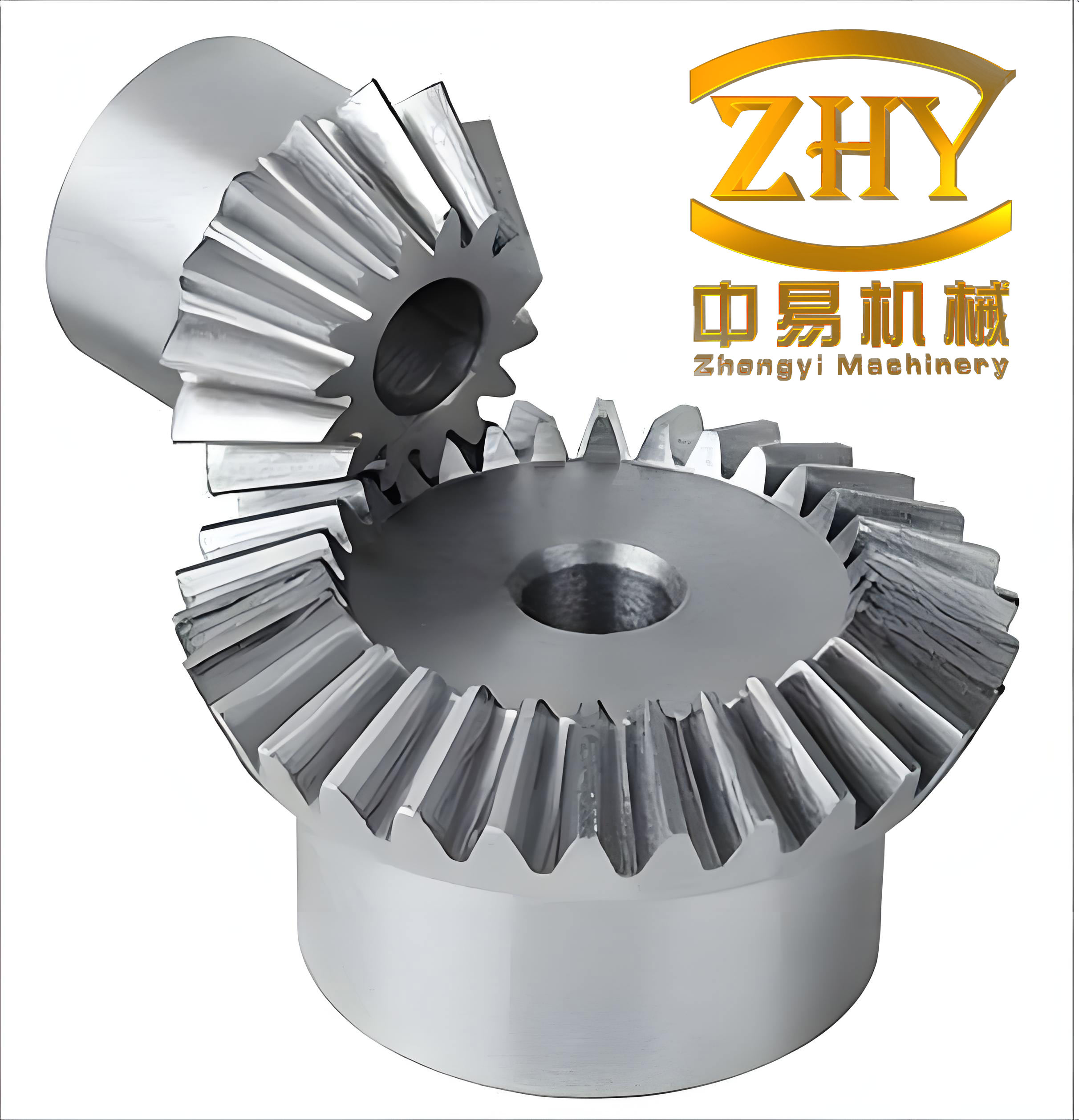
Straight bevel gears are fundamental mechanical transmission components, widely employed in locomotive powertrains, aerospace actuation systems, and heavy industrial machinery. As intersecting-axis gear drives, straight bevel gears transmit motion and power between shafts whose axes intersect at a specified angle, most commonly 90 degrees. The operational reliability of straight bevel gears directly determines the stability, safety, and service life of the entire mechanical system. In my research, I focus on the nonlinear dynamic behavior and chaos suppression of straight bevel gears, which has become a critical issue in modern mechanical engineering.
In locomotive applications, straight bevel gears are integral components of traction devices. They must continuously endure high torque loads, frequent starting and braking cycles, and complex variable operating conditions. The HXD1D electric locomotive, operating on the Lanzhou-Xinjiang railway, employs straight bevel gear pairs within its traction motor reduction device to achieve a 90-degree power transmission between the motor output shaft and the wheel axle. The internal structure of such a gearbox is illustrated below.
During service, straight bevel gears exhibit extremely complex dynamic characteristics due to the influence of various operating conditions. Potential faults such as tooth fracture, root cracks, tooth surface scoring, and pitting threaten the safe and stable operation of locomotives. Research by Wang and colleagues has demonstrated that both external excitations (prime mover torque, load reaction torque) and internal excitations (time-varying mesh stiffness, tooth transmission errors, meshing impact) significantly alter the contact state of gear pairs. The coupling of nonlinear factors including meshing backlash, tooth surface friction, time-varying mesh stiffness, and static transmission errors induces rich dynamic phenomena in the system, increasing both system uncertainty and control difficulty while significantly degrading transmission performance and operational stability. These nonlinear factors may drive straight bevel gears into chaotic states, exacerbating vibration. Chaos, as an undesirable phenomenon, leads to irregular oscillations, adversely affecting system performance, shortening mechanical equipment lifespan, and endangering high-speed and stable locomotive operation.
Given these challenges, traditional linear analysis approaches are no longer adequate for high-precision straight bevel gears. Only through thorough nonlinear vibration analysis can we design gear transmission systems with superior performance characteristics including high precision, low vibration, and low noise. The primary objective of my work is to develop an effective chaos control strategy for straight bevel gear transmission systems, leveraging the synergistic combination of fuzzy neural networks (FNN) and an improved particle swarm optimization (IPSO) algorithm.
2. Literature Review and Research Context
2.1 Dynamics Research on Straight Bevel Gears
Numerous scholars have investigated the dynamic characteristics of bevel gear systems. Wang Sanmin et al. studied a 7-degree-of-freedom (DOF) spiral bevel gear transmission system and obtained the torsional, lateral, and axial vibration displacements and velocities under different operating conditions. Their findings revealed that as mesh frequency varies, the system enters chaos through period-doubling bifurcation, while variations in support stiffness lead to chaotic vibration through quasi-periodic bifurcation. Wang Lihua and colleagues investigated bevel gear transmission systems without considering torsional vibrations, discovering that multiple steady-state responses exist when excitation frequency changes, including single-period harmonic responses, multi-period subharmonic responses, quasi-periodic responses, and chaotic responses.
Further research has expanded the model complexity. Qiu Huansong incorporated oil film effects into the analysis, examining how clearance variations influence the nonlinear characteristics of gear systems, concluding that time-varying clearance has a stronger effect on system amplitude and dynamic meshing force than constant clearance. Wang Shilong established a multi-DOF nonlinear dynamic model of spiral bevel gears considering time-varying friction force and friction coefficient. Li Chunyang studied the nonlinear dynamic phenomena of locked bevel gear systems with backlash, identifying both periodic and chaotic behaviors. Feng Gang investigated cracked bevel gear transmission systems, finding that cracks not only significantly affect system vibration response but also promote quasi-periodic and chaotic phenomena.
Zhao Ning developed an 8-DOF straight bevel gear transmission system and identified geometric transmission error as the dominant factor affecting gear vibration when manufacturing errors are excluded. The research established that vibration effects arising from mesh stiffness variations are strongly influenced by rotational speed and load. Wang Lihua’s work on spiral bevel gear systems demonstrated that varying mesh frequency produces multiple steady-state responses, with transitions between periodic responses occurring through quasi-periodic bifurcation.
2.2 Chaos Control in Gear Systems
Control methods can be broadly classified into feedback and non-feedback categories. Feedback control offers advantages including no requirement for precise system models, no alteration of system structure, and superior trajectory tracking capability. However, it demands relatively accurate mathematical models and explicit objective functions. Non-feedback control primarily works by introducing small external perturbations such as signals, constant biases, or weak parameter adjustments, making design and implementation straightforward but lacking guaranteed control stability. Li Weidong summarized fundamental chaos control methods as OGY methods, continuous feedback control (external force feedback and delayed feedback), adaptive control, and intelligent control approaches.
Recent research has applied these approaches to gear systems. Liu Xiaoning and colleagues used OGY methods to control chaos in single-stage gear systems with clearance nonlinearity. Chen Xuesen extended this work by incorporating time-varying mesh stiffness into single-stage gear models. Tian Yaping and colleagues implemented improved OGY control algorithms for high-dimensional non-smooth gear transmission systems. Wang Jingyue and co-authors employed three non-feedback methods to stabilize chaotic motion in gear systems considering backlash, time-varying mesh stiffness, and comprehensive mesh errors. Ghasem and colleagues established nonlinear time-varying dynamic models of spur gear pairs with backlash, time-varying stiffness, static transmission errors, and external excitations, subsequently applying sliding mode and adaptive sliding mode control strategies. Farshidianfar and Saghafi used Melnikov analysis to predict chaos in spur gear pairs and applied additional control excitation to eliminate chaos.
With advancing research, multi-DOF gear system chaos control has attracted increasing attention. Li Yinong and colleagues employed both fuzzy controllers and fuzzy PID controllers for chaos control in three-DOF gear transmission systems. Gao Yang utilized simplified RBF neural network controllers for chaos control of three-DOF gear systems. This evolution toward intelligent control methods reflects the recognition that the complexity of chaotic systems often makes precise analytical models difficult, if not impossible, to establish. Consequently, intelligent control strategies that rely solely on input-output data are becoming research hotspots, and my work follows this trajectory by applying fuzzy neural network control to straight bevel gears.
2.3 Fuzzy Neural Networks and Particle Swarm Optimization
Fuzzy neural networks combine the semantic interpretability of fuzzy logic with the adaptive learning capability of neural networks, providing exceptional advantages in handling uncertainty and nonlinearity. The inherent nonlinear mapping capability of neural networks, coupled with the logical reasoning functionality of fuzzy systems, enables more effective modeling of complex nonlinear relationships. Sun Zengqi and colleagues proposed a T-S model-based fuzzy neural network where parameter initialization can be guided by qualitative system knowledge, allowing rapid convergence to desired input-output relationships. Wang Xuewu and co-workers demonstrated that fuzzy neural networks synthesize the advantages of both constituent approaches while avoiding their respective drawbacks, making them broadly applicable in control systems.
Liu Ding and colleagues applied RBF neural network-based intelligent methods for chaos control without requiring analytical models of the controlled system. Various researchers have successfully applied fuzzy neural networks in gear thermal analysis, adaptive robot control, flexible structure vibration control, and unknown chaotic system synchronization. Li Xiuying proposed a T-S fuzzy neural network controller optimized by particle swarm optimization, achieving excellent control performance. Li Jiejia and colleagues optimized fuzzy RBF neural networks using improved PSO for furnace temperature control. Recent work by Xi Meng and collaborators introduced self-organizing fuzzy neural networks with hybrid learning algorithms for nonlinear system modeling.
In parallel, particle swarm optimization (PSO), first proposed by Kennedy and Eberhart in 1995, remains a cornerstone of intelligent optimization. While PSO offers structural simplicity and ease of parameter tuning, it suffers from premature convergence and local optima entrapment, particularly for high-dimensional complex objective functions. Numerous improvements have been proposed: Kuang Fangjun utilized Tent chaotic maps and artificial bee colony advantages, Wang Hao introduced global neighborhood search strategies, Fan Chengli incorporated auditing factors, and Yang Jingming developed multi-objective PSO variants. These enhancements share a common goal: improving convergence accuracy, convergence speed, and global search capability.
3. Nonlinear Dynamic Modeling of Straight Bevel Gears
3.1 Dynamic Excitation Mechanisms
In my study of straight bevel gears, I first needed to carefully characterize the dynamic excitation mechanisms. The time-varying mesh stiffness, which is one of the most significant internal excitations, arises from the periodic engagement and disengagement of gear tooth pairs. As the contact ratio of straight bevel gears typically falls between 1 and 2, the mesh alternates between single-tooth-pair and double-tooth-pair contact zones, causing periodic variations in the comprehensive mesh stiffness. The mesh stiffness function used in my analysis is expressed as:
$$k_h(t) = k_m + \sum_{l=1}^{N} k_{kl} \cos(l\Omega_h t + \phi_{kl})$$
where $k_m$ represents the mean mesh stiffness, $k_{kl}$ denotes the amplitude of the $l$-th harmonic component, $\Omega_h$ is the mesh frequency, and $\phi_{kl}$ represents the initial phase. For computational efficiency while maintaining adequate accuracy, I selected the first-order harmonic for my numerical analyses. The inherent geometric structure, machining precision, and assembly conditions of straight bevel gears generate transmission errors between actual and theoretical angular displacements. The comprehensive transmission error is expressed as:
$$e_n(t) = \sum_{l=1}^{N} A_l \cos(l\Omega_h t + \phi_l)$$
where $A_l$ denotes the amplitude of the $l$-th harmonic error component. The backlash function, which is fundamental to the non-smooth characteristics of straight bevel gears, is mathematically represented as:
$$f(\lambda, b_n) = \begin{cases} \lambda – b_n & \lambda > b_n \\ 0 & |\lambda| \leq b_n \\ \lambda + b_n & \lambda < -b_n \end{cases}$$
where $\lambda$ represents the relative torsional displacement along the line of action and $b_n$ is half of the backlash value. This piecewise linear function gives rise to three distinct meshing states for straight bevel gears: contact on the driving flank, separation (loss of contact), and contact on the coast flank.
The mesh damping coefficient for straight bevel gears critically influences energy dissipation during tooth engagement. It is calculated using the following formula:
$$c_h = 2\mu \sqrt{k_m m_e}$$
where $\mu$ is the mesh damping ratio typically ranging from 0.03 to 0.17, and $m_e$ represents the equivalent mass of the gear pair calculated as:
$$m_e = \frac{I_1 I_2}{r_1^2 I_2 + r_2^2 I_1}$$
3.2 Seven-DOF Dynamic Model
I developed a seven-degree-of-freedom dynamic model for straight bevel gears using the lumped mass method. The geometric parameters of the straight bevel gear pair analyzed in my research are summarized in Table 1.
| Parameter | Symbol | Pinion | Gear |
|---|---|---|---|
| Number of teeth | $z_1, z_2$ | 47 | 53 |
| Module (mm) | $m$ | 2 | |
| Pressure angle (°) | $\alpha_n$ | 20 | |
| Pitch cone angle (°) | $\delta_1, \delta_2$ | 41.57 | 48.43 |
| Cone distance (mm) | $R$ | 70.8 | |
| Face width (mm) | $b$ | 25 | |
| Reference diameter (mm) | $d_1, d_2$ | 94 | 106 |
| Speed ratio | $u$ | 1.13 | |
The model considers translational motions along three mutually perpendicular directions ($x_j$, $y_j$, $z_j$) for each gear ($j=1,2$) plus one torsional degree of freedom for each gear, resulting in eight equations originally. By introducing the relative displacement variable along the line of action, I reduced the system to seven efficiently coupled equations. The dynamic differential equations established through Newton’s second law are presented below for the translational degrees of freedom:
$$m_1 \ddot{y}_1 + c_{y1} \dot{y}_1 + k_{y1} y_1 = F_{y1}$$
$$m_1 \ddot{z}_1 + c_{z1} \dot{z}_1 + k_{z1} z_1 = F_{z1}$$
$$m_1 \ddot{x}_1 + c_{x1} \dot{x}_1 + k_{x1} x_1 = F_{x1}$$
for the pinion, and analogously for the gear:
$$m_2 \ddot{y}_2 + c_{y2} \dot{y}_2 + k_{y2} y_2 = -F_{y2}$$
$$m_2 \ddot{z}_2 + c_{z2} \dot{z}_2 + k_{z2} z_2 = -F_{z2}$$
$$m_2 \ddot{x}_2 + c_{x2} \dot{x}_2 + k_{x2} x_2 = -F_{x2}$$
where $m_1$, $m_2$ are the masses of pinion and gear respectively, $c_{ij}$ and $k_{ij}$ denote support damping and stiffness coefficients, and $F_{xi}$, $F_{yi}$, $F_{zi}$ represent the components of the dynamic meshing force along each direction. The relative displacement along the line of action, which accounts for tooth deformation and error excitation effects, takes the form:
$$\lambda = -\alpha_1 Y_1 – \alpha_2 Z_1 – \alpha_3 X_1 + r_1\theta_1 + \alpha_1 Y_2 + \alpha_2 Z_2 + \alpha_3 X_2 – r_2\theta_2 – e_n(t)$$
where $\alpha_1 = \cos\delta_1 \sin\alpha_n$, $\alpha_2 = \cos\delta_1 \cos\alpha_n$, $\alpha_3 = \cos\alpha_n$, and $r_1$, $r_2$ denote the base circle radii.
After extensive symbolic manipulation and substitution, I derived the complete set of governing equations and subsequently applied nondimensionalization to facilitate numerical analysis. The nondimensionalized state-space representation yields a system of 14 first-order differential equations, with the generalized displacement vector being $\mathbf{X} = [x_1, y_1, z_1, x_2, y_2, z_2, \lambda]^T$ and the corresponding velocity components. The key dimensionless parameters in this formulation include the mesh frequency ratio $\Omega = \Omega_h/\Omega_n$, the load coefficient $f_{pm} = F_{pm}/(\Omega_n^2 b_h m_e)$, the transmission error coefficient $f_e = \hat{e}_l / b_h$, and the time-varying stiffness ratio $a = k_{kl}/k_m$. The nondimensional mesh stiffness is expressed as:
$$k_h(\tau) = 1 + a\cos(\Omega\tau)$$
where $\tau = \Omega_n t$ is the dimensionless time. This complete formulation captures all the essential nonlinear characteristics of straight bevel gears and provides a solid foundation for the subsequent bifurcation analysis.
4. Bifurcation Characteristics of Straight Bevel Gears
4.1 Analysis Methodology
To investigate the bifurcation behavior of straight bevel gears, I employed numerical integration using the fourth-fifth order Runge-Kutta method with variable step size control. The analysis utilized bifurcation diagrams, phase portraits, and Poincaré maps to characterize the evolution of system dynamics. The constant parameter values adopted throughout the bifurcation analysis are presented in Table 2.
| Parameter | Value | Parameter | Value |
|---|---|---|---|
| $k_{x1}=k_{y1}=k_{z1}$ | 1.25 | $k_{x2}=k_{y2}=k_{z2}$ | 1.25 |
| $\xi_{x1}=\xi_{y1}=\xi_{z1}$ | 0.42 | $\xi_{x2}=\xi_{y2}=\xi_{z2}$ | 0.42 |
| $k_{h1}$ | 0.5 | $k_{h2}$ | 0.5 |
| $\xi_h$ | 0.06 | $\xi_{h1}=\xi_{h2}$ | 0.012 |
| $f_e$ | 0.2 | $b$ | 1.0 |
| $f_{pm}$ | 0.05 | $f_{pv}$ | 0 |
4.2 Bifurcation Response to Time-Varying Stiffness Coefficient
My analysis reveals remarkably rich dynamic behavior in straight bevel gears as the time-varying stiffness coefficient $a$ varies. Using the bifurcation parameter $a \in [0.1, 1.0]$, I observed the following sequence of dynamic transitions, summarized in Table 3.
| Parameter interval | Dynamic state | Bifurcation signature |
|---|---|---|
| $a \leq 0.3$ | Chaotic motion | Non-periodic point set on Poincaré map |
| $a \in (0.3, 0.35)$ | Transition from chaos to period-3 | Appearance of 3 closed loops |
| $a \in (0.35, 0.40)$ | Period-3 motion | Three discrete Poincaré points |
| $a \in (0.40, 0.427)$ | Period-6 motion | Period-doubling to period-6 |
| $a \in (0.43, 0.437)$ | Period-12 motion | Period-doubling from period-6 |
| $a \in (0.437, 0.441)$ | Period-24 motion | Further period-doubling |
| $a \in (0.441, 0.451)$ | Quasi-periodic motion | Hopf tori observed |
| $a > 0.451$ | Chaotic motion | Irregular phase trajectory |
At $a = 0.35$, I observed a sudden transition from chaotic motion to period-3 motion, representing a crisis bifurcation. The subsequent period-doubling cascade starting at $a = 0.40$ demonstrates the classic Feigenbaum route to chaos. This analysis of straight bevel gears clearly indicates that the stiffness fluctuation amplitude is a critical parameter significantly influencing system stability.
4.3 Bifurcation Response to Transmission Error Coefficient
Ranging the transmission error coefficient $f_e$ from 0 to 2.0, I mapped an extensive bifurcation diagram for straight bevel gears. The observed dynamic transitions are tabulated below (Table 4):
| Parameter interval | Dynamic state | Poincaré signature |
|---|---|---|
| $f_e < 0.1048$ | Period-1 motion | Single point |
| $f_e \in (0.1048, 0.133)$ | Period-2 motion | Two points |
| $f_e \in (0.133, 0.143)$ | Period-4 motion | Four points |
| $f_e \in (0.143, 0.149)$ | Period-8 motion | Eight points |
| $f_e \in (0.149, 0.2315)$ | Chaos (with Hopf bifurcation) | Closed curves and disorder |
| $f_e \in (0.2315, 0.2379)$ | Period-3 motion | Three points |
| $f_e \in (0.2379, 0.243)$ | Period-6 motion | Six points |
| $f_e \in (0.243, 0.378)$ | Chaotic motion | Non-periodic distribution |
| $f_e \in (0.378, 0.972)$ | Period-6 to Period-3 | Inverse period-doubling |
| $f_e \in (1.067, 1.077)$ | Quasi-periodic to Period-4 | Closed curve to 4 points |
| $f_e \in (1.09, 1.103)$ | Period-8 → 4 → 2 | Inverse period-doubling |
| $f_e > 1.467$ | Period-1 motion | Single point |
This extensive map of dynamical behavior underscores the sensitivity of straight bevel gears to transmission error excitation, which acts as a key trigger for chaotic vibration.
4.4 Bifurcation Response to Load Coefficient
Analyzing the effect of the load coefficient $f_{pm}$ across the range [0, 1.0], I observed several key transition phenomena. At very low loads ($f_{pm} < 0.00151$), the system maintains stable single-period motion. The load interval $f_{pm} \in (0.00248, 0.04)$ is dominated by chaotic motion interspersed with periodic windows. In the narrow band $f_{pm} \in (0.04001, 0.04023)$, I identified quasi-periodic motion containing a period-9 window. A period-6 to period-3 transition occurs in $f_{pm} \in (0.041, 0.0432)$ through inverse period-doubling bifurcation. Finally, for larger loads beyond $f_{pm} = 0.09$, straight bevel gears return to stable single-period motion. The load coefficient thus acts as a major bifurcation governor.
4.5 Bifurcation Response to Mesh Frequency Ratio
The mesh frequency ratio $\Omega$ fundamentally governs the dynamic behavior of straight bevel gears. In the interval $\Omega \in [0.5, 2.0]$, my analysis revealed the complete period-doubling route to chaos. Starting from single-period motion at $\Omega = 0.56$, the system transitions sequentially through period-2 at $\Omega = 0.65$, period-4 at $\Omega = 0.83$, and period-8 at $\Omega = 0.833$. A chaotic region dominates for $\Omega \in (0.843, 1.033)$. When $\Omega = 1.033$, I observed a boundary crisis leading to period-3 motion, followed by period-doubling to period-6 at $\Omega = 1.099$. After an additional chaotic window in $\Omega \in (1.105, 1.125)$, a complex finite transition leads through period-4 and period-2 states before stabilizing to single-period motion beyond $\Omega = 1.3$. The complete sequence for straight bevel gears is captured in Table 5.
| Frequency interval | Dynamic state |
|---|---|
| $\Omega = 0.56$ | Period-1 motion |
| $\Omega = 0.65$ | Period-2 motion |
| $\Omega = 0.83$ | Period-4 motion |
| $\Omega = 0.833$ | Period-8 motion |
| $\Omega \in (0.843, 1.033)$ | Chaotic motion |
| $\Omega = 1.066$ | Period-3 motion |
| $\Omega = 1.099$ | Period-6 motion |
| $\Omega \in (1.105, 1.125)$ | Chaotic motion |
| $\Omega = 1.253$ | Period-4 motion |
| $\Omega = 1.28$ | Period-2 motion |
| $\Omega = 1.3$ | Period-1 motion |
These comprehensive bifurcation analyses clearly demonstrate that straight bevel gears exhibit remarkably rich nonlinear behavior across wide parameter ranges. The identified chaotic regions represent dangerous operational zones that must be avoided or actively controlled in practical engineering applications.
5. Design of the IPSO-FNN Chaos Controller
5.1 Fuzzy Neural Network Structure
Based on the T-S fuzzy model, I designed a five-layer fuzzy neural network controller specifically tailored for chaos control of straight bevel gears. The network architecture comprises: (1) an input layer receiving two variables, (2) a fuzzification layer containing five fuzzy subsets per input, (3) a fuzzy rule layer computing rule activations, (4) a defuzzification layer normalizing the rule outputs, and (5) an output layer generating the control signal.
For the fuzzification layer, I adopted Gaussian membership functions:
$$\mu_i^m = \exp\left(-\frac{|x_i – C_{im}|^2}{b_{im}^2}\right), \quad i = 1,2; \quad m = 1,2,\ldots,5$$
where $C_{im}$ and $b_{im}$ are the center and width parameters of the $m$-th membership function for the $i$-th input, respectively. The five fuzzy subsets correspond to linguistic labels {very large, large, medium, small, very small} for each input dimension.
The rule layer computes the activation of each rule as the product of membership values:
$$\alpha_M = \mu_1^m \mu_2^m$$
The defuzzification layer normalizes rule activations to obtain firing strengths:
$$\bar{\alpha}_M = \frac{\alpha_M}{\sum_{j=1}^{M}\alpha_j}$$
Finally, the output layer produces the control perturbation through weighted summation:
$$U(k) = \sum_{i=1}^{M} \bar{\alpha}_i w_i$$
where $\mathbf{w} = [w_1, w_2, \ldots, w_M]^T$ is the weight matrix connecting the defuzzification layer to the output layer. The controller inputs are chosen as $d(k) = ||X(k) – X(k-1)||$ and $d(k-1) = ||X(k-1) – X(k-2)||$, representing the Euclidean distances between consecutive points on the Poincaré section. This innovative selection of controller inputs capitalizes on the geometric structure of chaotic attractors in straight bevel gears.
5.2 Controller Configuration and Control Flow
The complete closed-loop control strategy operates as follows. The straight bevel gear system is allowed to evolve freely for 200 iterations, reaching a steady chaotic or undesirable state on the Poincaré section. At this point, the controller begins generating perturbations $\Delta\Omega$ that are added to the system’s frequency ratio (or load coefficient). The perturbation is applied through:
$$\Omega_{e} = \Omega_0 + U(k)$$
where $\Omega_0$ is the original parameter value. The control system continuously monitors the state of straight bevel gears through the Poincaré section distance signals and adjusts the perturbation to steer the system toward the desired target orbit. The desired distance $d^*$ between adjacent Poincaré points serves as the reference for the target periodic orbit.
5.3 Improved Particle Swarm Optimization
The parameter optimization of the fuzzy neural network controller is a high-dimensional, multimodal optimization problem. Standard PSO algorithms often suffer from premature convergence and insufficient solution precision, which are unacceptable for chaos control applications where small parameter deviations can dramatically alter control performance. To address these challenges, I developed an improved PSO algorithm incorporating several enhanced mechanisms.
5.3.1 Chaotic Population Initialization
I adopted a Piecewise chaotic map to generate the initial population positions, leveraging the ergodicity and randomness of chaotic sequences to achieve more uniform coverage of the solution space. The Piecewise map is defined as:
$$x_{n+1} = \begin{cases} \frac{x_n}{q} & 0 \leq x_n < q \\ \frac{x_n – q}{0.5 – q} & q \leq x_n < 0.5 \\ \frac{1 – q – x_n}{0.5 – q} & 0.5 \leq x_n < 1 – q \\ \frac{1 – x_n}{q} & 1 – q \leq x_n < 1 \end{cases}$$
where $q$ is the control parameter (typically set to 1). This approach effectively prevents particle clustering in localized regions of the parameter space, thereby reducing the risk of premature convergence for the chaos controller optimization.
5.3.2 Adaptive Learning Factors
The learning factors $c_1$ and $c_2$ represent the “step sizes” of particles toward their personal best and global best positions, respectively. I designed a nonlinear adaptation strategy that dynamically adjusts these factors throughout the optimization process:
$$c_1 = 2\sin\left(\frac{\pi}{2}\left(1 – \frac{t}{T}\right)\right), \quad c_2 = 2\sin\left(\frac{\pi}{2}\left(\frac{t}{T}\right)\right)$$
During early iterations ($c_1 > c_2$), particles are guided more strongly by their own historical experience, promoting broad exploration of the solution space. As iterations progress, $c_2$ increases relative to $c_1$, steering the swarm toward the global optimum neighborhood for refined exploitation. This synergistic adaptation significantly enhances convergence accuracy for optimizing the fuzzy neural network parameters used in controlling straight bevel gears.
5.3.3 Adaptive Inertia Weight
I implemented a time-varying nonlinear inertia weight using a tangent-based decay function:
$$w(t) = (w_{Max} – w_{Min})\tan\left(0.875\left(1 – \left(\frac{t}{T}\right)^k\right)\right) + w_{Min}$$
where $w_{Max} = 0.9$, $w_{Min} = 0.1$, and $k = 0.6$. This formulation maintains high inertia weight in early iterations for extensive global search, then gradually reduces $w$ to emphasize fine-grained local exploration around promising regions, a critical feature for handling the high-dimensional parameter space in the FNN chaos controller design for straight bevel gears.
5.3.4 Lévy Flight with Dynamic Centroid Migration
To further enhance swarm diversity and global search ability, I incorporated a Lévy flight mechanism into the position update equation. Lévy flights are characterized by occasional long-distance jumps interspersed with short-distance movements, enabling particles to escape local optima. The flight step length is governed by the Lévy distribution:
$$s = \frac{\mu}{|v|^{1/\beta}}$$
where $\mu \sim N(0, \sigma_\mu^2)$, $v \sim N(0, 1)$, $\beta = 1.5$, and:
$$\sigma_\mu = \left[\frac{\Gamma(1+\beta)\sin(\pi\beta/2)}{\Gamma((1+\beta)/2)2^{(\beta-1)/2}}\right]^{1/\beta}$$
My key innovation involves replacing the traditional worst-solution-partner Lévy strategy with a global-best-directed scheme. This “dynamic centroid migration” approach gradually shifts the search gravity center from dispersed exploration toward the global optimum neighborhood as iterations progress. The position update becomes:
$$p_{is}(t+1) = b_2 p_{is}(t) + b_1 p_{gbest} + 0.01s \cdot (p_{is}(t) – p_{gbest})$$
Finally, I designed a Bernoulli-distribution-based selection mechanism that stochastically chooses between the standard PSO update and the Lévy flight update with probability $p = 0.5$. This coordination strategy balances exploration and exploitation throughout the optimization process for the FNN controller parameters.
5.4 Benchmark Function Validation
I validated the improved PSO algorithm using eight standard benchmark functions, including Ackley, Alpine, Eggholder, Griewank, Levy, Rastrigin, Schaffer, and Weierstrass functions. These test functions present various optimization challenges including multimodality, local optima traps, narrow valleys, and high-dimensional complexity. The algorithmic parameters used in validation were: population size = 150, maximum iterations = 1500, and problem dimension = 20. The comparative results are summarized in Table 6.
| Function | Standard PSO | Improved PSO | Theoretical Optimum |
|---|---|---|---|
| Ackley | 5.0574e-04 | 8.8817e-16 | 0 |
| Alpine | 0.1453189 | 6.0014e-141 | 0 |
| Eggholder | 795.01 | 959.64 | -959.6407 |
| Griewank | 1.1504e-07 | 0 | 0 |
| Levy | 0.0902181 | 3.0395e-07 | 0 |
| Rastrigin | 8.1888471 | 0 | 0 |
| Schaffer | -0.9951158 | -1 | -1 |
| Weierstrass | 2.5038663 | 0 | 0 |
The improved PSO achieved the theoretical optimum value on four of the eight test functions and attained significantly better precision on the remaining functions. In particular, the Eggholder function (a notoriously difficult multimodal function) saw a 17% improvement over the standard PSO. These results conclusively demonstrate that the improved PSO possesses superior global search capability, faster convergence, and stronger ability to escape local optima—all essential attributes for optimizing the fuzzy neural network chaos controller parameters for straight bevel gears.
6. Chaos Control Simulation Results for Straight Bevel Gears
6.1 Control Implementation
Using the improved PSO algorithm to optimize the fuzzy neural network controller parameters, I conducted comprehensive chaos control simulations on the seven-DOF straight bevel gear dynamic model. In all simulations, the FNN controller parameters were constrained to the range $[-3, 3]$ for weights $w$, and centers $c$, and widths $b$ of the membership functions. The swarm size was set to 150 particles with a maximum of 100 iterations. The controller was activated after 200 system iterations, allowing the system to fully develop its undesired dynamic state before control intervention. The target orbit was specified according to the desired periodic motion.
6.2 Control of Chaotic Motion to Period-1 Orbit
I first analyzed the control of chaotic motion to a stable period-1 orbit. The system parameters were set to those in Table 2 with stiffness coefficient $a = 0.25$ and initial frequency ratio $\Omega_0 = 0.862$, placing the system in a chaotic state characterized by a folded and intertwined phase trajectory and non-periodic Poincaré points. After control activation, the output perturbation from the FNN controller rapidly drove the system into a stable single-period orbit. The simulation results demonstrated convergence within approximately 13 perturbation steps, with the Poincaré map reducing to a single discrete point. The controller output perturbation stabilized quickly to a very small constant value, confirming the efficiency of the control strategy.
Table 7 presents the optimized FNN controller parameters for period-1 control:
| Weight $w$ | Widths $b_{1m}$ and $b_{2m}$ | Centers $C_{1m}$ and $C_{2m}$ |
|---|---|---|
| -1.7350 | -1.5721, -1.2846 | -1.6693, -1.7799 |
| -0.1285 | -1.6599, -1.3353 | -0.8814, -0.6160 |
| -1.7931 | -0.9319, -0.3782 | -0.9916, -1.2283 |
| -0.2182 | -1.2521, -0.7416 | -0.6149, -1.1715 |
| -0.3479 | -1.5100, -0.5805 | -0.1482, 0.6168 |
6.3 Control of Chaotic Motion to Period-2 Orbit
Using identical system parameters and initial conditions, I next investigated control of the same chaotic state of straight bevel gears to a stable period-2 orbit. The controller successfully stabilized the system within approximately 4 perturbation iterations, with the Poincaré section exhibiting exactly two discrete points. The perturbation signal again converged rapidly to a small constant value, demonstrating fast and precise control. The optimized parameters for this case are provided in Table 8.
| Weight $w$ | Widths $b_{1m}$ and $b_{2m}$ | Centers $C_{1m}$ and $C_{2m}$ |
|---|---|---|
| -0.0803 | -1.4886, 0.9841 | 0.1473, 0.1163 |
| 0.4621 | -0.4757, 0.0399 | 0.2704, 1.0648 |
| 0.3427 | 1.6503, -0.1176 | -0.6700, -1.2135 |
| 0.0148 | -0.8108, 0.2946 | -0.4539, -1.0073 |
| -0.5040 | 0.4740, 0.0034 | -0.1899, -0.1414 |
6.4 Control of Chaotic Motion to Period-4 Orbit
Continuing with the same initial chaotic state, I implemented control to achieve a period-4 orbit. The controller achieved stable period-4 motion within approximately 10 perturbation steps. The Poincaré section confirmed exactly four discrete points, and the perturbation magnitude remained minimal. Table 9 lists the optimized controller parameters.
| Weight $w$ | Widths $b_{1m}$ and $b_{2m}$ | Centers $C_{1m}$ and $C_{2m}$ |
|---|---|---|
| -0.3808 | -1.9091, -2.4368 | -1.3317, -3.0000 |
| -0.8313 | -0.5714, -2.1608 | -3.0000, -2.4170 |
| -2.6842 | -1.0141, -0.2008 | -2.2337, -1.6978 |
| -1.0908 | -2.7536, -0.0543 | -1.9870, -1.5736 |
| -1.0023 | -1.4612, -1.0337 | -2.0165, -2.5512 |
6.5 Control of Multi-Periodic Motion to Period-4 Orbit
Beyond controlling chaotic states, I also investigated suppressing multi-periodic motions of straight bevel gears to simpler target orbits. Using the same system parameter set and an initial frequency ratio of $\Omega_0 = 1.23$, the system exhibited multi-periodic behavior with multiple scattered Poincaré points. When the controller was activated, the system rapidly transitioned into a stable period-4 orbit within approximately 6 perturbation steps. The control perturbation signal demonstrated fast convergence to a constant small value, confirming efficient stabilization. These results are significant because they demonstrate that the IPSO-FNN approach is not limited to chaotic suppression but can also re-shape multi-periodic responses in straight bevel gears.
6.6 Control of Multi-Periodic Motion to Period-2 and Period-1 Orbits
Using an initial frequency ratio of $\Omega_0 = 1.256$, the system was in a multi-periodic state. My controller effectively drove this state to a stable period-2 orbit within approximately 5 perturbation steps, with the Poincaré section exhibiting exactly two discrete points. Additionally, by adjusting the controller parameters, the same initial multi-periodic state was successfully controlled to a stable single-period orbit within approximately 17 perturbation iterations. Table 10 summarizes the control performance metrics for straight bevel gears under various frequency ratio parameter values.
| Initial state | Initial $\Omega$ | Target orbit | Convergence time (iterations) | Poincaré points |
|---|---|---|---|---|
| Chaotic | 0.862 | Period-1 | 13 | 1 |
| Chaotic | 0.862 | Period-2 | 4 | 2 |
| Chaotic | 0.862 | Period-4 | 10 | 4 |
| Multi-periodic | 1.230 | Period-4 | 6 | 4 |
| Multi-periodic | 1.256 | Period-2 | 5 | 2 |
| Multi-periodic | 1.256 | Period-1 | 17 | 1 |
6.7 Load-Activated Chaos Control
To generalize the control approach, I also tested the controller with the load coefficient $f_{pm}$ as the control parameter. I selected a different set of constant parameters ($k_{x1}=k_{y1}=k_{z1}=k_{y2}=k_{z2}=k_{x2}=1.25$; $\xi_{x1}=\xi_{y1}=\xi_{z1}=\xi_{x2}=\xi_{y2}=\xi_{z2}=0.42$; $\xi_h=0.06$; $\xi_{h1}=\xi_{h2}=0.012$; $f_e=0.025$; $\Omega=1$; $f_{pv}=0$; $b=1$; $k_{h1}=k_{h2}=0.5$; $\alpha=0.15$). With an initial load coefficient $f_{pm} = 0.002$, the system exhibited chaos. After activating the IPSO-FNN controller, the system was stabilized to a period-2 orbit within approximately 20 perturbation steps. This demonstrates the versatility and robustness of the control approach for straight bevel gears across different perturbation parameters, confirming that the control method is not limited to frequency manipulation but applies equally well to load-based control.
Additionally, I tested the control strategy when the initial state was quasi-periodic. With initial load coefficient $f_{pm} = 0.016$, where the Poincaré section showed closed-curve structure, the controller successfully stabilized the system to period-2 motion within approximately 5 perturbation steps. The controller parameter values used for this case matched those in Table 8, suggesting a certain degree of universality in the optimized parameters for similar dynamic states in straight bevel gears.
7. Discussion and Conclusions
Through my comprehensive research on chaos control of straight bevel gears, I have established a complete theoretical and computational framework encompassing dynamic modeling, bifurcation analysis, intelligent controller design, and numerical validation.
The dynamic modeling work demonstrated that a seven-DOF lumped parameter model of straight bevel gears, incorporating time-varying mesh stiffness, backlash, transmission errors, damping, and load effects, accurately captures the essential nonlinear behaviors of the physical system. My bifurcation analyses revealed that straight bevel gears exhibit remarkably diverse dynamic responses across parameter variations. Key findings include:
(1) The time-varying stiffness coefficient $a$ induces a sequence of transitions from chaos through period-3, period-6, period-12, and period-24 motions, ultimately returning to chaos. This pattern reflects the classic period-doubling route with interspersed crisis events. The stiffness fluctuation amplitude in straight bevel gears is therefore a critical design parameter that should be controlled to maintain stable periodic operation.
(2) The transmission error coefficient $f_e$ acts as a powerful bifurcation trigger, generating an extensive roadmap of periodic, quasi-periodic, and chaotic attractors across the range [0, 2.0]. Chaos-dominated regions exist for $f_e \in (0.16, 0.4)$ and $f_e \in (1.1, 1.2)$, values which should be avoided in practical design of straight bevel gears.
(3) The load coefficient $f_{pm}$ exhibits a bifurcation structure where chaos dominates the low-to-moderate load range, but stable periodic motion resumes for sufficiently high loads ($f_{pm} > 0.09$). This suggests that maintaining adequate load levels can help avoid chaotic vibration in straight bevel gears.
(4) The mesh frequency ratio $\Omega$ profoundly governs the dynamics, with chaotic windows appearing between $0.843$ and $1.033$ and between $1.105$ and $1.125$. These frequency bands represent dangerous operating zones for straight bevel gears in locomotive applications and should be avoided through appropriate design and speed selection.
For controller design, my work proved that the fuzzy neural network with a five-layer structure provides an effective paradigm for chaos suppression in straight bevel gears. The network’s ability to approximate complex nonlinear mappings between Poincaré-map-derived distance signals and control perturbations enables model-independent chaos control. This is a critical advantage because most engineering implementations of straight bevel gears lack precise analytical models under operational conditions.
My improved particle swarm optimization algorithm has shown excellent capability in optimizing the FNN controller parameters. The key innovations—piecewise chaotic initialization, adaptive learning factors, tangent-based nonlinear inertia weight, and the dynamic centroid migration Lévy flight mechanism—collectively overcome the inherent limitations of standard PSO. Benchmarking on eight difficult test functions confirmed substantially better convergence speed, solution precision, and global search achievement compared to the standard algorithm.
The numerical simulation results conclusively demonstrate that the IPSO-FNN hybrid controller effectively controls chaotic, quasi-periodic, and multi-periodic motions of straight bevel gears to desired target orbits. All control tasks—whether targeting period-1, period-2, or period-4 motion—were achieved with minimal control effort and rapid convergence times ranging from 4 to 20 perturbation steps. The controlled systems exhibited stable Poincaré maps with discrete points exactly matching the specified target period, confirming the precision and reliability of the proposed control scheme for straight bevel gears.
8. Future Research Directions
While my research has established a robust theoretical foundation for chaos control of straight bevel gears, several promising directions remain for future investigation:
(1) The current model considers simplified nonlinear factors. Future work should incorporate additional realistic effects including thermo-elastohydrodynamic lubrication coupling, tooth surface wear evolution, and bearing clearance variations to enhance model fidelity for straight bevel gears operating under extreme conditions.
(2) Experimental validation of the proposed control scheme on physical test rigs is essential. I plan to design experiments using accelerometers and torque sensors on a bevel gear test bench to measure vibration response and verify the predicted bifurcation and chaos suppression phenomena in straight bevel gears.
(3) Real-time implementation of the IPSO-FNN controller on digital signal processing hardware should be explored to assess computational efficiency and practical control latency in straight bevel gear applications.
(4) Extending the proposed control methodology to related gear types such as spiral bevel gears and hypoid gears would provide broader industrial applicability of the chaos control strategy I developed.
(5) Further improvement of the IPSO algorithm, possibly by hybridizing it with other metaheuristic techniques such as differential evolution or teaching-learning-based optimization, may unlock even greater parameter optimization capability for the FNN-based control of straight bevel gears.
In conclusion, my work provides a comprehensive and systematic investigation into the nonlinear dynamics and chaos suppression of straight bevel gears. The IPSO-FNN control framework offers a promising intelligent approach for ensuring vibration-free operation of straight bevel gears in critical applications such as locomotive transmission systems, paving the way for enhanced reliability, safety, and service life of mechanical power transmission equipment.