
1 Introduction
In the context of promoting green development and energy conservation, gear transmission is advancing toward lightweight, high-efficiency, and low-noise directions. Herringbone gear transmission offers advantages such as compact structure, smooth operation, low axial force, and high load-carrying capacity, making it widely used in aerospace, marine, and metallurgical fields. The double helical star gear transmission device is the core component of a Geared Turbofan (GTF) engine. Its service conditions are complex with multiple excitation sources. The comprehensive friction coefficient at the rolling-sliding interface, normal contact force distribution, and relative sliding velocity directly affect the frictional power loss and meshing efficiency of the gear system. Therefore, researching the meshing efficiency calculation and influence laws of the herringbone gear system, and mastering the macro-micro parameter optimization design method, are key measures to improve the meshing efficiency of the gear system. The time-varying meshing stiffness, tooth surface friction, meshing phase, and meshing error are the main internal dynamic excitations affecting the meshing efficiency of the herringbone gear system. Considering multiple internal dynamic excitations comprehensively and establishing a multi-degree-of-freedom coupled dynamic model can accurately solve the dynamic meshing force required for meshing efficiency calculation. In high-speed and heavy-load gear transmissions such as large marine gearboxes and GTF engines, the meshing power loss of gear pairs significantly impacts the system transmission efficiency. The frictional power loss is the main component of meshing power loss. Therefore, it is necessary to study the meshing efficiency calculation of double helical star gear systems and the macro-micro parameter optimization based on efficiency improvement.
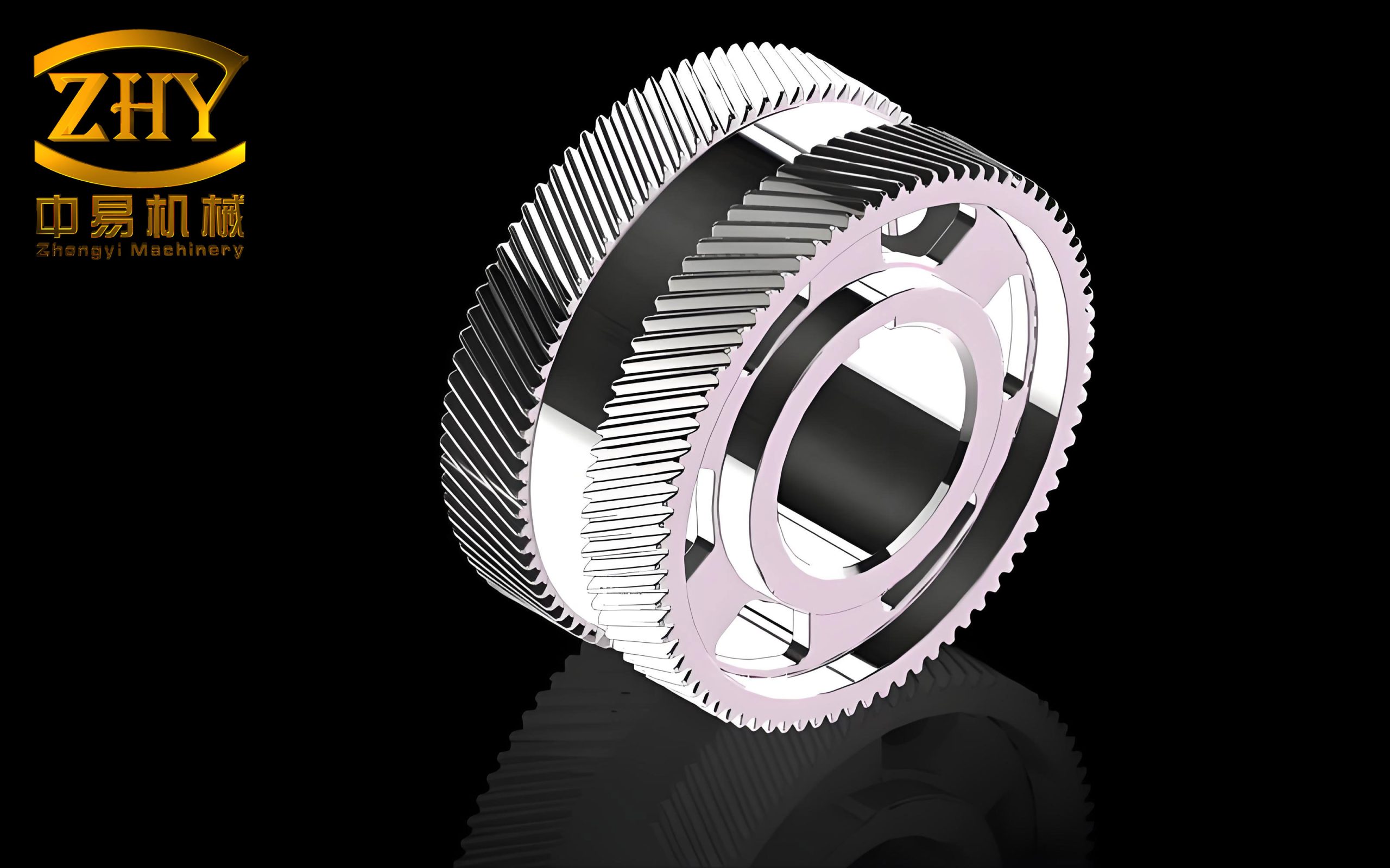
2 Friction Excitation Analysis of Herringbone Gear Pairs Based on Mixed Elastohydrodynamic Lubrication
2.1 Contact Ratio Calculation of Modified Herringbone Gear Pairs
The double helical star gear system consists of a sun gear, five star gears, an internal ring gear, and a carrier. Power is input through the sun gear, split into five star gears, and converged to the internal ring gear for output, with the carrier fixed. The geometric parameters of the scaled prototype are presented in Table 1. The rated input power is 2000 kW and the input speed is 7500 r/min.
| Parameter | Sun gear | Star gear | Ring gear |
|---|---|---|---|
| Number of teeth z | 34 | 31 | 96 |
| Normal module mn / mm | 2 | ||
| Normal pressure angle αn / (°) | 22.5 | ||
| Helix angle β / (°) | 30 | ||
| Overall tooth width Bz / mm | 58 | ||
| Gap width Bt / mm | 10 | ||
| Normal modification coefficient xn | 0.1016 | 0.1235 | 0.3485 |
During operation, because of manufacturing errors, thermal–elastic deformation, and load deformation, tooth modification is applied to the sun gear and star gears. The modification amount is Ca = Cf = 10 μm, the modification length is La = Lf = 1 mm, and a parabolic modification curve is adopted. The transverse contact ratios for the internal and external meshing herringbone gear pairs are calculated as follows.
For the internal meshing gear pair:
$$ \varepsilon_{\alpha i}=\frac{\sqrt{r_{e1}^{2}-r_{b1}^{2}}-r_{w1}\sin\alpha_{t}+\sqrt{r_{s2}^{2}-r_{b2}^{2}}-r_{w2}\sin\alpha_{t}}{P_{bt}} $$
For the external meshing gear pair:
$$ \varepsilon_{\alpha e}=\frac{\sqrt{r_{e1}^{2}-r_{b1}^{2}}-r_{w1}\sin\alpha_{t}+\sqrt{r_{s2}^{2}-r_{b2}^{2}}+r_{w2}\sin\alpha_{t}}{P_{bt}} $$
The longitudinal contact ratio is:
$$ \varepsilon_{\beta}=\frac{B\sin\beta}{\pi m_{n}} $$
The total contact ratios are εγi = 3.184 for the internal meshing pair and εγe = 3.138 for the external meshing pair.
2.2 Time-Varying Contact Line Length and Kinematic Parameters
Based on the mesh motion characteristics of the herringbone gear pair, the double helical gear can be equivalently decomposed into left and right helical gears coupled through the gap. According to the relationship between the base helix angle βb and the critical helix angle β0 = arctan(εαPbt/B), the contact line length of a single tooth pair is derived for three cases. For the case where βb < β0, the variation is given by:
$$ l(t)=\begin{cases} 2v_{0}t\sin\beta_{b}, & t\in[0,t_{1}] \\ 2B, & t\in[t_{1},t_{2}] \\ 2(B+P_{bt}\varepsilon_{\alpha}-v_{0}t)\sin\beta_{b}, & t\in[t_{2},t_{3}] \\ 0, & t\in[t_{3},T] \end{cases} $$
Similarly, expressions for the cases βb = β0 and βb > β0 are derived. The total time-varying contact line length is obtained by summing the lengths of all meshing tooth pairs:
$$ L_{z}(t)=\sum_{i=1}^{N} l_{i}(t) $$
The contact line length of the herringbone gear pair changes periodically, and the difference between the maximum and minimum values is small, resulting in smooth transmission and low vibration and noise.
The radius of curvature, entrainment velocity, relative sliding velocity, and slide-roll ratio along the mesh line are derived. The distance between the pitch point P and any meshing point K on the line of action is:
$$ PK = r_{b1}(\tan\alpha_{t1}-\tan\alpha_{t}) $$
The transverse radii of curvature are:
$$ \begin{cases} R_{t1}=N_{1}P+PK = r_{b1}\tan\alpha_{t1} \\ R_{t2}=N_{2}P+PK = r_{b1}\tan\alpha_{t}(1\mp i) \end{cases} $$
where the upper sign is for external meshing and the lower sign for internal meshing. The comprehensive radius of curvature is:
$$ R_{z}=\frac{R_{n1}R_{n2}}{R_{n2}\pm R_{n1}} $$
The tangential velocity components at any meshing point are:
$$ \begin{cases} v_{t1}=\omega_{1}R_{t1}=\frac{\pi n_{1}}{30}r_{b1}\tan\alpha_{t1} \\ v_{t2}=\omega_{2}R_{t2}=\frac{\pi n_{2}}{30}r_{b1}\tan\alpha_{t}(1\mp i) \end{cases} $$
Consequently, the relative sliding velocity vs, entrainment velocity ve, and slide-roll ratio ζ are:
$$ \begin{cases} v_{s}=|v_{t1}-v_{t2}| \\ v_{e}=(v_{t1}+v_{t2})/2 \\ \zeta=2(v_{t1}-v_{t2})/(v_{t1}+v_{t2}) \end{cases} $$
The relative sliding velocity is zero at the pitch line and changes direction on both sides of it. The internal meshing gear pair has a larger variation of entrainment velocity along the tooth height direction compared to the external meshing pair.
2.3 Friction Coefficient Calculation under Mixed EHL
Under heavy-load conditions, the herringbone gear transmission operates in the mixed elastohydrodynamic lubrication (EHL) regime. The total tooth load Fd is shared by the lubricant film and asperity contacts. The comprehensive friction coefficient is:
$$ \mu = \gamma \mu_{e} + (1-\gamma)\mu_{b} $$
where γ is the oil film load-sharing ratio, μe is the film friction coefficient obtained from Xu’s regression formula, and μb is the asperity contact friction coefficient taken as 0.12. The oil film load-sharing ratio is calculated using Hu and Zhu’s empirical formula:
$$ \gamma = \frac{1.21\lambda^{0.64}}{1+0.37\lambda^{1.26}} $$
where λ is the film thickness ratio determined by the minimum film thickness from Dowson-Higginson equation:
$$ h_{min} = 2.65 \frac{\alpha^{0.54}(\eta_{0}v_{e})^{0.7}R_{z}^{0.43}}{\varpi^{0.13}E^{0.03}} $$
Using the lubrication parameters listed in Table 2, the minimum film thickness, film thickness ratio, oil film load-sharing ratio, and comprehensive friction coefficient are calculated for both internal and external meshing herringbone gear pairs respectively.
| Parameter | Value |
|---|---|
| Pressure-viscosity coefficient α / (m2·N−1) | 1.68×10⁻⁸ |
| Dynamic viscosity η0 / (Pa·s) | 0.0347 |
| Comprehensive elastic modulus E / Pa | 2.264×10¹¹ |
| Surface roughness of driving gear σ1 / μm | 0.6 |
| Surface roughness of driven gear σ2 / μm | 0.6 |
The analysis reveals that the film thickness ratio lies between 1 and 3, confirming the mixed EHL condition. The internal meshing pair exhibits better lubrication characteristics than the external meshing pair. Near the pitch point, the friction coefficient approaches zero because pure rolling occurs. For the internal meshing pair, the friction coefficient at the tooth root of the driving gear is larger than at the tooth tip; for the external meshing pair, the friction coefficient decreases at positions far from the pitch point due to thermal effects reducing oil viscosity.
2.4 Friction Force and Friction Torque Analysis
Using the contact-line segmentation method, each meshing tooth pair is discretized into small segments of length ΔL. The normal load acting on the j-th segment of the i-th meshing pair is:
$$ F_{nij}(t) = \frac{\Delta L}{L_{z}(t)} F_{z}(t) $$
The friction force on that segment is:
$$ F_{fij}(t) = \mu_{ij}(t) F_{nij}(t) $$
Since the friction direction reverses when the contact line crosses the pitch line, the contact line is divided into two portions relative to the pitch line. The total friction force and the friction torque on the driving and driven gears are obtained by summation. The time-varying friction force and friction torque of the internal and external meshing herringbone gear pairs are obtained, and the results show periodic variation. For the external meshing pair, the friction torques on the driving and driven gears are similar because the tooth numbers are comparable. For the internal meshing pair, the friction torque on the ring gear is significantly larger than that on the pinion due to the larger friction moment arm.
3 Dynamic Modeling and Dynamic Meshing Force Analysis of the Double Helical Star Gear System
3.1 Time-Varying Meshing Stiffness
Under the mixed EHL state, the total time-varying meshing stiffness is composed of the boundary-lubrication stiffness and the EHL stiffness. The latter includes the oil film squeezing stiffness. The single-tooth time-varying meshing stiffness is expressed as:
$$ k_{m}(t) = k_{m}'(t) L(t) $$
The total time-varying meshing stiffness is obtained by summing over all meshing tooth pairs:
$$ K(t) = \sum_{i=1}^{N} k_{i}(t) $$
The mean meshing stiffness in the mixed EHL state is:
$$ k_{m}(t) = \gamma k_{e}(t) + (1-\gamma)k_{b} $$
The EHL stiffness considers the gear tooth body deformation and oil film deformation in series:
$$ \frac{1}{k_{e}} = \frac{1}{k_{p}} + \frac{1}{k_{g}} + \frac{1}{k_{f}} $$
The oil film stiffness is derived from the derivative of load with respect to the minimum film thickness:
$$ k_{f}(t) = \frac{\partial F}{\partial h_{min}} = \frac{2.65\alpha^{0.54}(\eta_{0}v_{e})^{0.7}R_{z}^{0.43}L_{z}^{0.13}}{13 E^{0.03}} \cdot \frac{1}{h_{min}^{14/13}} $$
The boundary-lubrication stiffness is calculated from an empirical formula. The time-varying meshing stiffness of the internal (star gear–ring gear) and external (sun gear–star gear) meshing herringbone gear pairs are obtained with mean values of 8.353×10⁸ N/m and 8.220×10⁸ N/m, respectively, as shown in Figure 1.
| Method | Mean stiffness / (N/m) | Error vs. LTCA |
|---|---|---|
| Mixed EHL analytical method | 1.32×10⁹ | 5.71% |
| Loaded tooth contact analysis (LTCA) | 1.25×10⁹ | — |
The comparison verifies the reliability of the present approach.
3.2 Meshing Phase and Meshing Error
The meshing phase relationships among the five star gears are defined based on the number of teeth and installation angles. The phase differences between the internal meshing gear pairs and the external meshing gear pairs are given by:
$$ \begin{cases} \gamma_{ri} = \psi_{i} z_{p}/2\pi \pm \psi_{i} z_{p}/2\pi \\ \gamma_{si} = \psi_{i} z_{s}/2\pi \end{cases} $$
The phase difference between the internal and external meshing gear pairs is:
$$ \gamma_{sr} = 0.5 z_{p}/z_{r} \ \text{or} \ 0 $$
depending on whether the number of star gear teeth is even or odd.
The meshing errors include manufacturing eccentricity errors of the sun gear, star gears, and ring gear, as well as tooth profile errors. These errors are equivalent to the mesh line direction and superposed linearly. For example, the equivalent meshing error of the sun gear eccentricity is:
$$ e_{s}^{E,i} = E_{s}\sin(\omega_{s}t + \delta_{s} \mp \alpha_{w} + \psi_{i})\cos\beta_{b} $$
The comprehensive meshing error for each gear pair is represented as the sum of individual components.
3.3 Equations of Motion of the Lumped-Parameter Model
Using the lumped-parameter method, a bending-torsion-axial coupling dynamic model of the double helical star gear system is established. The model has 56 degrees of freedom, including the translational motions along the x, y, z axes and the torsional rotation about the z axis for both left and right sides of the sun gear, five star gears, and ring gear. The relative displacements along the line of action for the external and internal meshing gear pairs are:
$$ \delta_{spi}^{L} = (x_{s}^{L}-x_{pi}^{L})\sin\varphi_{spi}\cos\beta_{b} + (y_{s}^{L}-y_{pi}^{L})\cos\varphi_{spi}\cos\beta_{b} + (z_{s}^{L}-z_{pi}^{L})\sin\beta_{b} + r_{bs}\theta_{s}^{L} + r_{bpi}\theta_{pi}^{L} – e_{spi}^{L} $$
$$ \delta_{rpi}^{L} = (x_{pi}^{L}-x_{r}^{L})\sin\varphi_{rpi}\cos\beta_{b} + (y_{pi}^{L}-y_{r}^{L})\cos\varphi_{rpi}\cos\beta_{b} + (z_{pi}^{L}-z_{r}^{L})\sin\beta_{b} + r_{bpi}\theta_{pi}^{L} – r_{br}\theta_{r}^{L} – e_{rpi}^{L} $$
The dynamic meshing forces are expressed as:
$$ \begin{cases} F_{spi}^{L} = k_{spi}^{L}(t)\delta_{spi}^{L} + c_{spi}^{L}\dot{\delta}_{spi}^{L} \\ F_{rpi}^{L} = k_{rpi}^{L}(t)\delta_{rpi}^{L} + c_{rpi}^{L}\dot{\delta}_{rpi}^{L} \end{cases} $$
where the meshing damping is calculated from the average stiffness and equivalent masses. The differential equations of motion for the sun gear, star gears, and ring gear are derived according to Newton’s second law. The equations for the degrees of freedom of the sun gear are:
$$ \begin{cases} m_{s}\ddot{x}_{s}^{L} + k_{sx}^{L}x_{s}^{L} + c_{sx}^{L}\dot{x}_{s}^{L} + k_{sx}^{LR}(x_{s}^{L}-x_{s}^{R}) + c_{sx}^{LR}(\dot{x}_{s}^{L}-\dot{x}_{s}^{R}) – \sum_{i=1}^{5}F_{spi}^{L}\sin\varphi_{spi}\cos\beta_{b} = 0 \\ m_{s}\ddot{y}_{s}^{L} + k_{sy}^{L}y_{s}^{L} + c_{sy}^{L}\dot{y}_{s}^{L} + k_{sy}^{LR}(y_{s}^{L}-y_{s}^{R}) + c_{sy}^{LR}(\dot{y}_{s}^{L}-\dot{y}_{s}^{R}) – \sum_{i=1}^{5}F_{spi}^{L}\cos\varphi_{spi}\cos\beta_{b} = 0 \\ m_{s}\ddot{z}_{s}^{L} + k_{sz}^{L}z_{s}^{L} + c_{sz}^{L}\dot{z}_{s}^{L} + k_{sz}^{LR}(z_{s}^{L}-z_{s}^{R}) + c_{sz}^{LR}(\dot{z}_{s}^{L}-\dot{z}_{s}^{R}) – \sum_{i=1}^{5}F_{spi}^{L}\sin\beta_{b} = 0 \\ J_{s}\ddot{\theta}_{s}^{L} + k_{s\theta}^{L}\theta_{s}^{L} + c_{s\theta}^{L}\dot{\theta}_{s}^{L} + k_{s\theta}^{LR}(\theta_{s}^{L}-\theta_{s}^{R}) + c_{s\theta}^{LR}(\dot{\theta}_{s}^{L}-\dot{\theta}_{s}^{R}) – \sum_{i=1}^{5}F_{spi}^{L}r_{bs}\cos\beta_{b} + T_{in}^{L}/2 = 0 \end{cases} $$
A similar set of equations is formulated for each star gear and the ring gear. The overall system equation is:
$$ \mathbf{M}\ddot{\mathbf{X}} + \mathbf{C}\dot{\mathbf{X}} + \mathbf{K}\mathbf{X} = \mathbf{F} $$
where M, C, and K are the mass, damping, and stiffness matrices, and F is the force vector including friction excitations.
3.4 Dynamic Meshing Force Analysis
The time-varying meshing stiffness is expanded into a Fourier series:
$$ k(t) = a_{0} + \sum_{n=1}^{\infty}[a_{n}\cos(n\omega_{m}t) + b_{n}\sin(n\omega_{m}t)] $$
where ωm is the mesh frequency. The differential equations are solved using a variable-step Runge-Kutta method to obtain the dynamic responses. The dynamic meshing forces are then calculated from the relative displacements and velocities combined with the meshing stiffness and damping. The time-domain results of the internal and external meshing herringbone gear pairs are presented in Figure 2 for both left and right sides.
| Gear pair | Left mean / kN | Right mean / kN | Phase difference |
|---|---|---|---|
| rp1–rp5 (internal) | 8.31 | 8.29 | in phase |
| sp1–sp4 (external) | 8.65 | 8.63 | phase shifted |
The dynamic meshing forces of the left and right side gears exhibit similar variation patterns, fluctuating periodically around the static contact force. The internal and external meshing gear pairs have different phases. The frequency spectrum shows peaks at 125 Hz (sun gear rotation frequency), 137 Hz (star gear rotation frequency), 44 Hz (ring gear rotation frequency), and the mesh frequency of 4250 Hz with superharmonics at multiples thereof.
The influence of oil film stiffness, internal meshing stiffness, and external meshing stiffness on the dynamic meshing force is also investigated. When the oil film stiffness is included, the overall meshing stiffness decreases compared to the case without it. The relative error of the dynamic meshing force due to the oil film stiffness is shown to be larger for the internal meshing pair than for the external meshing pair. Furthermore, as the internal or external meshing stiffness increases, the range of fluctuation of the dynamic meshing force increases, with the decrease being more significant for the correspondingly named meshing force.
4 Meshing Efficiency Calculation and Influencing Factor Analysis of the Herringbone Gear System
4.1 Meshing Efficiency Calculation
The sliding friction power loss is calculated using the contact-line segmentation method. For the j-th segment of the i-th meshing tooth pair at time t, the sliding friction power loss is:
$$ P_{sij}^{L}(t) = \mu_{ij}^{L}(t)F_{nij}^{L}(t)v_{sij}(t) $$
The total sliding friction power loss of the double helical star gear system is:
$$ P_{s}^{ALL}(t) = \sum_{i=1}^{5}P_{si}^{sun-star}(t) + \sum_{i=1}^{5}P_{si}^{star-ring}(t) $$
The rolling friction power loss is calculated using Hamrock and Jacobson’s formula:
$$ P_{r} = \frac{b\varepsilon}{\cos\beta_{b}}\cdot\frac{90 v_{r} h}{\alpha} $$
where the mean rolling velocity vr and the mean film thickness h are:
$$ v_{r} = 0.2094 n_{1} r_{1}\sin\alpha_{t}\left(\frac{z_{2}}{z_{1}}\mp 1\right)^{0.125} $$
$$ h = 3.07\frac{\alpha^{0.57}(\eta_{0}v_{r})^{0.71}R_{z}^{0.4}}{E^{0.11}\varpi^{0.3}} $$
The meshing efficiency is defined as:
$$ \eta = \frac{P_{in} – P_{s}^{ALL} – P_{r}^{ALL}}{P_{in}} $$
The total friction power loss curve obtained by the contact-line method is shown in Figure 3, along with the result from Niemann’s formula. The sliding friction power loss accounts for nearly all of the total mesh power loss, indicating the rolling friction loss is negligible under heavy loads. The contact-line method yields a time-varying power loss due to the time-varying dynamic meshing force, whereas Niemann’s formula gives a constant value of 16.57 kW. The mean meshing efficiency calculated by the present method is 99.08%, compared to 99.17% from Niemann’s formula, which demonstrates the rationality of the calculation.
4.2 Influence of Macro Parameters on Meshing Efficiency
4.2.1 Number of Teeth
While keeping other parameters unchanged, the influence of the number of teeth on the meshing efficiency is studied. The tooth number combinations are listed in Table 3.
| Set | 1 | 2 | 3 | 4 |
|---|---|---|---|---|
| Sun gear teeth z1 | 24 | 29 | 34 | 39 |
| Star gear teeth z2 | 41 | 36 | 31 | 26 |
| Ring gear teeth z3 | 106 | 101 | 96 | 91 |
The mean dynamic meshing force decreases with an increasing number of teeth, which leads to a smaller normal contact force per unit length and hence reduced sliding friction loss. Consequently, the meshing efficiency increases with the number of teeth.
4.2.2 Module
As the module mn increases from 1.5 mm to 3 mm, the gear radius increases, the relative sliding velocity at the meshing entry point increases, and the contact line length increases, resulting in a larger sliding friction power loss and a lower meshing efficiency, as shown in Figure 4.
4.2.3 Tooth Width
The overall tooth width Bz varies from 48 mm to 78 mm. The longitudinal contact ratio increases, and the total contact line length increases. In the heavy-load condition, the contact force per unit length decreases, so the sliding friction loss decreases slightly and the meshing efficiency increases slightly.
4.2.4 Helix Angle
From 20° to 35°, both the transverse and longitudinal contact ratios increase, leading to more tooth pairs in mesh and a lower load per tooth. Therefore, the meshing efficiency slightly increases with an increasing helix angle, as shown in Figure 5.
4.2.5 Pressure Angle
For pressure angles ranging from 17.5° to 25°, although the contact force increases, the friction coefficient decreases with an increasing pressure angle because the oil temperature rises and the viscosity drops. The overall sliding friction loss decreases with an increasing pressure angle, and the meshing efficiency increases accordingly.
4.2.6 Modification Coefficient
The modification coefficient distribution has a significant influence on the meshing efficiency under high torque. Unreasonable modification coefficient distribution can increase the difference between entry and exit sliding velocities, leading to larger sliding friction loss and lower efficiency. Proper allocation is beneficial for efficiency improvement.
4.3 Influence of Micro Parameters on Meshing Efficiency
4.3.1 Surface Roughness
When the surface roughness increases from 0.2 μm to 0.8 μm, the oil film load-sharing ratio decreases, the friction coefficient increases, and thus the meshing efficiency decreases. The efficiency drops from above 99.6% at σ = 0.2 μm to approximately 98.5% at σ = 0.8 μm.
4.3.2 Profile Modification Amount and Length
With the increase of profile modification amount C from 8 μm to 14 μm, the transverse contact ratio decreases, the meshing region becomes smaller, the relative sliding velocity at the entry point decreases, and the friction coefficient also decreases; hence, the meshing efficiency increases. The same trend is found with the modification length L varying from 0.6 mm to 1.2 mm, as shown in Figure 6.
4.4 Summary of Influencing Laws and Efficiency Improvement Methods
Table 5 summarizes the variation trends of meshing efficiency with respect to macro and micro parameters.
| Parameter | Meshing efficiency | Parameter | Meshing efficiency |
|---|---|---|---|
| Number of teeth z | ↑ | Surface roughness σ | ↓ |
| Module mn | ↓ | Modification amount C | ↑ |
| Tooth width Bz | ↑ | Modification length L | ↑ |
| Helix angle β | ↑ | Modification coefficient xn | related to allocation |
| Pressure angle αn | ↑ |
According to these findings, efficiency improvement methods include adopting a smaller module with a larger tooth number under strength requirements, selecting larger tooth width and helix angle while considering machining cost and difficulty, choosing a larger pressure angle under strength constraints, rationally allocating modification coefficients, and reducing surface roughness through proper manufacturing and heat-treatment processes.
5 Macro and Micro Parameter Optimization of the Herringbone Gear System Based on Efficiency Improvement
5.1 Optimization Model
Based on the influence analysis in the previous chapter, the design variables are selected as the numbers of teeth z1, z2, z3, the normal module mn, the normal pressure angle αn, the modification coefficients xn1, xn2, xn3, and the profile modification parameters C and L. The design variable vector is:
$$ \mathbf{X} = [z_{1}, z_{2}, z_{3}, x_{n1}, x_{n2}, x_{n3}, m_{n}, \alpha_{n}, C, L]^{T} $$
Three objective functions are established:
- Minimization of total mass:
$$ M = \rho\cdot\frac{\pi}{4}\left[B_{z}(d_{a1}^{2}+nd_{a2}^{2}+d_{f3}^{2}-d_{a3}^{2}) – B_{t}(d_{t2}^{2}-d_{t1}^{2})\right] $$
$$ F_{1}(\mathbf{X}) = \frac{M}{M_{0}} $$
- Maximization of meshing efficiency:
$$ \eta = 1 – \frac{1}{T P_{in}}\int_{0}^{T}P_{s}^{ALL}(t)\,dt $$
$$ F_{2}(\mathbf{X}) = \frac{\eta_{0}}{\eta} $$
- Minimization of static transmission error peak-to-peak value:
$$ P = \max(E) – \min(E), \quad E = \frac{F_{z}}{K\cos\beta_{b}} $$
$$ F_{3}(\mathbf{X}) = \frac{P}{P_{0}} $$
The total objective function is formed using the weighted sum method:
$$ F(\mathbf{X}) = w_{1}F_{1}(\mathbf{X}) + w_{2}F_{2}(\mathbf{X}) + w_{3}F_{3}(\mathbf{X}) $$
The weights are chosen as w1 = 0.3, w2 = 0.4, and w3 = 0.3 to balance the three objectives.
The constraints include:
- Assembly condition for uniform planet distribution:
$$ \begin{cases} z_{1}+z_{2} = 5k_{1} \\ z_{3}-z_{2} = 5k_{2} \end{cases} \quad (k_{1}, k_{2} \in \mathbb{Z}) $$
- Range constraints on teeth numbers:
$$ \begin{cases} 20 \leq z_{1}, z_{2} \leq 60 \\ 80 \leq z_{3} \leq 200 \end{cases} $$
- Modification parameters: 0 ≤ C ≤ 30 μm, 0 ≤ L ≤ 2 mm
- Transmission ratio tolerance:
$$ \left|\frac{i – i_{0}}{i_{0}}\right| \leq 0.05 $$
- Standard module set: mn ∈ {1, 1.5, 2, 2.5, 3} mm
- Standard pressure angle set: αn ∈ {15°, 17.5°, 20°, 22.5°, 25°}
- Modification coefficient ranges:
$$ \begin{cases} 0.05 \leq x_{n1}, x_{n2} \leq 0.50 \\ 0.20 \leq x_{n3} \leq 0.80 \end{cases} $$
- No undercutting condition:
$$ \frac{z}{2}\sin^{2}\alpha_{n} – h_{a}^{*} – x_{n} \geq 0 $$
- Center distance tolerance:
$$ \left|\frac{a – a_{0}}{a_{0}}\right| \leq 0.05 $$
- Contact fatigue strength safety factor SH ≥ SHmin
- Bending fatigue strength safety factor SF ≥ SFmin
5.2 Optimization Procedure Using Genetic Algorithm
The optimization problem is solved using the MATLAB built-in genetic algorithm function ga. The mathematical formulation is expressed as:
$$ \begin{cases} \text{vars: } \mathbf{X} = [x_{1}, x_{2}, \dots, x_{10}] \\ \min: F(\mathbf{X}) = w_{1}F_{1}(\mathbf{X}) + w_{2}F_{2}(\mathbf{X}) + w_{3}F_{3}(\mathbf{X}) \\ \text{s.t.: } \mathbf{lb} \leq \mathbf{X} \leq \mathbf{ub}, \ \mathbf{A}\mathbf{X} \leq \mathbf{b}, \ c(\mathbf{X}) \leq 0, \ c_{eq}(\mathbf{X}) = 0 \end{cases} $$
Key parameters of the genetic algorithm are: population size = 100, number of generations = 100, crossover probability = 0.8, mutation probability = 0.2, and tolerance = 1×10⁻¹⁰.
5.3 Optimization Results and Evaluation
The optimal design variables obtained by the genetic algorithm are given in Table 6.
| Parameter | Before | After |
|---|---|---|
| Sun gear teeth z1 | 34 | 41 |
| Star gear teeth z2 | 31 | 39 |
| Ring gear teeth z3 | 96 | 119 |
| Module mn / mm | 2 | 1.5 |
| Pressure angle αn / (°) | 22.5 | 25 |
| Modification coefficient xn1 | 0.1016 | 0.2243 |
| Modification coefficient xn2 | 0.1235 | 0.2576 |
| Modification coefficient xn3 | 0.3485 | 0.4983 |
| Modification amount C / μm | 10 | 16.51 |
| Modification length L / mm | 1 | 1.689 |
The optimization results are summarized in Table 7.
| Objective | Before | After | Change |
|---|---|---|---|
| Mass M / kg | 11.7910 | 9.9699 | −15.44% |
| Mean meshing efficiency η | 0.9908 | 0.9936 | +0.28% |
| Static transmission error P / μm | 2.6274 | 2.1318 | −18.86% |
After optimization, the total mass decreases by 15.44%, the mean meshing efficiency increases by 0.28%, and the static transmission error peak-to-peak value decreases by 18.86%. The optimized design achieves the objectives of low mass, high efficiency, and low noise, improving the transmission performance and stability of the herringbone gear system.
The safety factors before and after optimization are compared in Table 8.
| Component | Contact safety factor SH | Bending safety factor SF | ||
|---|---|---|---|---|
| Before | After | Before | After | |
| Sun gear | 1.61 | 1.57 | 1.71 | 1.61 |
| Star gear | 1.76 | 1.69 | 1.57 | 1.49 |
| Ring gear | 1.82 | 1.75 | 2.04 | 1.92 |
All safety factors meet the minimum requirements, confirming the validity of the optimal design.
6 Conclusions and Outlook
6.1 Conclusions
In this thesis, the meshing efficiency calculation and macro-micro parameter optimization of a double helical star gear system are comprehensively studied. The main conclusions are as follows:
- The friction excitation of herringbone gear pairs is analyzed based on the mixed EHL theory. The time-varying contact line length, comprehensive radius of curvature, entrainment velocity, and relative sliding velocity are derived. The comprehensive friction coefficient under mixed lubrication is obtained. The time-varying friction force and friction torque are calculated using the contact-line segmentation method.
- A bending-torsion-axial coupling dynamic model of the double helical star gear system is established using the lumped-parameter method. The dynamic meshing forces are obtained for both internal and external meshing herringbone gear pairs. The influence of oil film stiffness and meshing stiffness on the dynamic meshing force is investigated. The results show that the left and right side dynamic meshing forces follow similar patterns, while the internal and external gear pairs exhibit phase differences.
- The total frictional power loss and meshing efficiency of the herringbone gear system are calculated. The results are verified against Niemann’s formula. The parametric study reveals that the meshing efficiency increases with the number of teeth, tooth width, helix angle, pressure angle, profile modification amount, and modification length, while it decreases with an increase in module and surface roughness.
- A multi-objective optimization model of the herringbone gear system is established with the objectives of minimizing mass, maximizing meshing efficiency, and minimizing the static transmission error peak-to-peak value. The model is solved using a genetic algorithm. The optimization results show that the mass is reduced by 15.44%, the meshing efficiency is improved by 0.28%, and the static transmission error is reduced by 18.86%, while all strength constraints are satisfied.
6.2 Outlook
Further research directions include incorporating installation errors, backlash, and external excitations into the dynamic model for more accurate dynamic meshing force predictions. In addition, the manufacturing and test verification of the optimized herringbone gear system would be valuable to further validate the results.