
Herringbone gears are widely used in aviation engines as key transmission components due to their high load-carrying capacity, smooth meshing, and ability to eliminate axial thrust. However, their complex geometry, narrow clearance grooves, and stringent surface integrity requirements make grinding a challenging process. In my research, I focus on optimizing the form grinding process of herringbone gears, developing a predictive model for grinding forces, and bridging the gap between design and manufacturing through a collaborative digital tool. The central idea is to expand the usable grinding wheel diameter by borrowing space from adjacent tooth slots and the empty groove, thereby increasing grinding efficiency while maintaining accuracy. I also investigate the micro-interaction between abrasive grains and the workpiece, and establish a stage-wise grinding force model. This article presents my findings, supported by analytical derivations, numerical simulations, and experimental validations.
1. Introduction and Research Motivation
In modern aviation transmission systems, the demand for high power-to-weight ratio pushes designers to reduce the size and mass of herringbone gears. However, this conflicts with the need for larger grinding wheels to achieve higher material removal rates and better surface quality. In conventional practice, the grinding wheel diameter is limited by the width of the herringbone gear’s central clearance groove. A smaller groove reduces weight but restricts the wheel size, leading to frequent wheel dressing and replacement, lower productivity, and inconsistent quality. To resolve this contradiction, I propose a novel borrowing grinding method that allows the grinding wheel to utilize the adjacent tooth slot space and the opposite tooth slot space during machining. This method is quantified by a dimensionless borrowing coefficient, which enables engineers to determine whether a given herringbone gear can be ground with a larger wheel without interference.
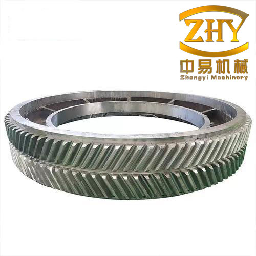
The core contributions of my research are threefold. First, I establish geometric models for the maximum grinding wheel diameter under two borrowing scenarios: empty-groove borrowing and tooth-slot borrowing. Second, I derive a grinding force prediction model that accounts for the stochastic nature of abrasive grains and the three stages of grain-workpiece interaction. Third, I develop a practical grinding process software that integrates borrowing judgment and collaborative design, making the theoretical findings directly usable on the shop floor.
2. Borrowing Grinding Method for Herringbone Gears
2.1 Classification of Grinding Wheel Borrowing
In the form grinding of herringbone gears, the grinding wheel approaches the tooth slot from the groove side. Traditionally, the wheel diameter is limited by the straight-line distance between the wheel center and the opposite tooth flank. My proposed method exploits the spatial geometry of the herringbone gear by allowing the wheel to extend into three types of spaces: the opposite tooth slot, the opposite adjacent tooth slot, and the central empty groove. These three configurations are illustrated conceptually in my analysis. The first configuration, borrowing the opposite tooth slot, requires the wheel to traverse a space equivalent to one pitch along the pitch circle. The second configuration, borrowing the opposite adjacent tooth slot, uses the space of the tooth slot that is one pitch away from the current slot. The third configuration is simply the traditional use of the empty groove. By borrowing these spaces, the effective limiting boundary for the wheel periphery is pushed outward, allowing a larger wheel diameter for the same nominal gear dimensions.
2.2 Geometric Modeling of Key Parameters
To quantify the feasibility of borrowing grinding, I develop a geometric model on the pitch cylinder surface. Let \(L\) be the width of the empty groove, \(\beta\) the helix angle, \(R\) the pitch circle radius, \(m_n\) the normal module, and \(Z\) the number of teeth. The arc length \(ab\) along the pitch circle between two reference points can be expressed as:
$$
\frac{\pi m_n}{\sin\beta} = L \cdot K
$$
Here \(K\) is defined as the borrowing coefficient, which represents the number of pitch intervals spanned by the wheel’s lateral displacement. Based on extensive numerical simulations, the valid range of \(K\) is found to be between 0 and 3. When \(K \ge 1.75\), the wheel and gear profiles become separated and no further borrowing is possible. The boundary functions and pitch interval relationships are shown in Table 1.
| Borrowing coefficient range | Wheel behavior | Applicability |
|---|---|---|
| [0, 0.25) | Borrows opposite tooth slot | Rare, small \(\beta\) |
| [0.25, 0.75) | Interference with opposite flank | Not allowed |
| [0.75, 1.25) | Borrows opposite adjacent tooth slot | Common for \(\beta \approx 15^{\circ}\)–\(35^{\circ}\) |
| [1.25, 1.75) | Interference with adjacent flank | Not allowed |
| [1.75, \(\infty\)) | No interference | Rare, large \(\beta\) |
Taking into account the tooth side clearance \(J_t\) and safety margin \(\delta\), the lower and upper boundaries of the borrowing coefficient can be refined as:
$$
K_a = 0.75 – \frac{J_t}{S_p} + \delta, \quad K_b = 1.25 + \frac{J_t}{S_p} – \delta
$$
where \(S_p\) is the circular pitch. The interval \([0.75, 1.25)\) is the most significant range because it provides a clear condition for borrowing the adjacent tooth slot without interference. My formulation enables a direct evaluation of whether a given herringbone gear can be ground with an enlarged wheel.
3. Maximum Grinding Wheel Diameter Modeling
3.1 Empty-Groove Borrowing Model
For the empty-groove borrowing configuration, the maximum wheel diameter \(D\) can be determined from the geometric relationship in the triangle \(dco’\). Let \(R_u\) be the tip circle radius, and \(L\) the groove width. The auxiliary distances are:
$$
ab = L \tan\beta, \quad ac = \frac{L}{\cos\beta}, \quad ao = \sqrt{R_u^2 + ab^2}, \quad co = \sqrt{R_u^2 + L^2}
$$
Applying the law of cosines in triangle \(aoc\):
$$
\cos\angle cao = \frac{ac^2 + ao^2 – co^2}{2 \cdot ac \cdot ao}
$$
The distance \(cd\) is then obtained from triangle \(acd\):
$$
cd = \sqrt{ac^2 + ad^2 – 2 \cdot ac \cdot ad \cdot \cos\angle cao}
$$
where \(ad = ao – R_u\). Since the line \(gd\) and \(co’\) are collinear, the angle \(\angle dco’\) is:
$$
\angle dco’ = \frac{\pi}{2} + \angle gcd
$$
with
$$
\angle gcd = \arcsin\left(\frac{gd}{cd}\right), \quad gd = ad \cdot \cos\angle gda, \quad \angle gda = \frac{2\pi}{Z}
$$
Finally, in triangle \(dco’\), the maximum wheel diameter \(D\) is:
$$
D = \frac{2 \cdot cd \cdot h \cdot \cos(\angle dco’) + \sqrt{cd^2 + h^2 + 2 \cdot cd \cdot h \cdot \cos(\angle dco’)}}{\cos(\angle dco’)}
$$
where \(h\) is a known vertical offset. This equation defines the largest wheel that can pass through the empty groove without touching the gear body.
3.2 Tooth-Slot Borrowing Model
When the grinding wheel borrows the opposite adjacent tooth slot, the maximum diameter \(D_{\text{Max}}\) is calculated in triangle \(fco’\). The geometry becomes more complex because the line \(cd\) and \(cf\) are not collinear, and the tooth trace on the base cylinder is twisted. I introduce the correction term \(\overline{df’}\) to account for the deformation of the tooth line. The relevant equations are:
$$
\overline{ee’} = w \tan\beta \left(1 – \frac{R_u}{R} \right), \quad \overline{en} = \frac{w}{\cos\beta}
$$
$$
\overline{e’n} = \sqrt{\overline{en}^2 + \overline{ee’}^2 + 2 \cdot \overline{en} \cdot \overline{ee’} \cdot \cos\beta}
$$
In triangle \(fde’\), the depth \(df’\) is found as:
$$
\overline{df’} = \frac{\overline{ne’} \cdot \sin(\angle ne’d)}{\cos(\beta – \angle ne’d)}
$$
The angular deviation due to tooth curvature is:
$$
\angle fcf’ = \arctan\left(\frac{\Delta f}{\overline{df’} + cd}\right)
$$
where \(\Delta f\) is the radial drop of point \(f\) caused by the helical deformation:
$$
\Delta f = \overline{df’} \cdot \sin\beta + R_u – \sqrt{R_u^2 – \left(\overline{df’} \cdot \sin\beta\right)^2}
$$
Combining all intermediate terms, I obtain the maximum wheel diameter for tooth-slot borrowing:
$$
D_{\text{Max}} = \frac{2 \cdot \overline{f’c} \cdot h \cdot \cos(\angle f’co’) + \sqrt{\overline{f’c}^2 + h^2 + 2 \cdot \overline{f’c} \cdot h \cdot \cos(\angle f’co’)}}{\cos(\angle f’co’)}
$$
where
$$
\overline{f’c} = \frac{U \cdot \overline{df’} + V \cdot cd}{\cos(\angle fcf’)}
$$
The coefficients \(U\) and \(V\) are correction functions derived from extensive contact simulations. They are expressed as:
$$
U = \cos(2\pi K) \cdot |K – 1|, \quad V = \frac{L \cdot m_n \cdot \sin\beta}{L + m_n \cdot \sin\beta}
$$
These functions correct the lateral offset and the nonlinearity of the boundary curve, respectively. I validated the coefficient functions numerically, and the maximum deviation was below 5%.
3.3 Compensation for Wheel Thickness and Center-Over Grinding
In actual machining, the wheel has a finite thickness, and the wheel must be lifted over the center of the gear to grind the full tooth flank. This requires an additional vertical space \(D_E\). The compensation is given by:
$$
D_E = C_{cn} \sin\beta, \quad L_E = C_{cn} \sin\beta \cos\beta
$$
where
$$
C_{cn} = \frac{S_u}{2\pi R_u} \cdot \frac{\pi R_u}{Z} – \frac{S_u}{2} \cdot \frac{1}{\cos\alpha_u}
$$
After incorporating these corrections, the final maximum diameter formulas become:
$$
D = \frac{2 \cdot (cd – D_E) \cdot h \cdot \cos(\angle dco’) + \sqrt{(cd – D_E)^2 + h^2 + 2 \cdot (cd – D_E) \cdot h \cdot \cos(\angle dco’)}}{\cos(\angle dco’)}
$$
$$
D_{\text{Max}} = \frac{2 \cdot (\overline{f’c} – D_E) \cdot h \cdot \cos(\angle f’co’) + \sqrt{(\overline{f’c} – D_E)^2 + h^2 + 2 \cdot (\overline{f’c} – D_E) \cdot h \cdot \cos(\angle f’co’)}}{\cos(\angle f’co’)}
$$
These corrected models allow process planners to determine the maximum permissible wheel diameter precisely, avoiding trial-and-error dressing and reducing setup time.
3.4 Validation Using Contact Simulation
To verify my analytical models, I conducted solid contact simulations for twelve typical herringbone gear specifications. The simulation setup incorporated the gear geometry, wheel dimensions, and the exact relative positions. Two types of interference were analyzed: thickness interference and profile interference. I compared the calculated maximum diameters \(D\) and \(D_{\text{Max}}\) with the simulated values. Table 2 presents a summary for representative gears.
| Gear ID | \(K\) | Borrowing | \(D\) (mm) | \(D’\) (mm) | Error (%) | \(D_{\text{Max}}\) (mm) | \(D’_{\text{Max}}\) (mm) | Error (%) |
|---|---|---|---|---|---|---|---|---|
| 1 | 0.721 | Yes | 48.745 | 49.195 | 0.915 | 64.334 | 68.000 | 5.391 |
| 2 | 0.721 | Yes | 48.938 | 48.186 | 1.573 | 59.037 | 63.000 | 6.290 |
| 5 | 1.158 | Yes | 90.617 | 93.961 | 3.559 | 118.422 | 128.159 | 7.598 |
| 6 | 1.158 | Yes | 82.469 | 82.514 | 0.055 | 100.243 | 102.660 | 2.354 |
| 7 | 0.749 | Yes | 53.629 | 53.979 | 0.648 | 53.691 | 52.000 | 3.252 |
| 8 | 0.749 | Yes | 52.872 | 52.462 | 0.782 | 52.764 | 55.000 | 4.065 |
| 9 | 0.796 | Yes | 56.588 | 57.341 | 1.313 | 67.520 | 67.000 | 0.776 |
| 10 | 0.796 | Yes | 57.320 | 57.728 | 0.707 | 68.150 | 68.000 | 0.221 |
The average errors for \(D\) and \(D_{\text{Max}}\) are 3.43% and 3.74%, respectively. These values confirm that the analytical models are accurate and conservative enough for practical use. I also verified the intermediate variable \(D_E\) (the lifting distance) through simulation; the average relative error was only 4.45%.
3.5 Experimental Validation on a CNC Gear Grinder
I further validated the maximum diameter models by performing contact experiments on a Klingelnberg CNC gear grinding machine. Two additional herringbone gears (Gear 13 and Gear 14) were prepared. The wheel was made of resinoid material to avoid damaging the ground flanks. For Gear 13, the computed empty-groove maximum diameter was \(D = 149.8084\) mm, while the actual model wheel diameter was set to 150 mm, resulting in an error of 0.13%. For Gear 14, the tooth-slot borrowing maximum diameter was \(D_{\text{Max}} = 54.7443\) mm, and the model wheel diameter was 55 mm, yielding an error of 0.46%. These tests demonstrate that the model is not only accurate but also robust in a real machining environment.
3.6 Discussion on Practical Benefits
Table 3 shows the efficiency improvement achieved by tooth-slot borrowing for several herringbone gears.
| Gear ID | \(K\) | \(D\) (mm) | \(D_{\text{Max}}\) (mm) | Improvement (%) |
|---|---|---|---|---|
| 1 | 0.821 | 48.745 | 64.334 | 31.981 |
| 2 | 0.821 | 48.938 | 59.037 | 20.636 |
| 5 | 1.158 | 90.617 | 118.422 | 30.684 |
| 6 | 1.158 | 82.469 | 100.243 | 21.552 |
| 7 | 0.749 | 53.629 | 53.691 | 0.116 |
| 8 | 0.749 | 52.872 | 52.764 | -0.204 |
| 9 | 0.796 | 56.588 | 67.520 | 19.319 |
| 10 | 0.796 | 57.320 | 68.150 | 18.894 |
Gears 5 and 6 exhibit remarkable improvements of about 30% and 21%, respectively. However, for Gears 7 and 8, the improvement is negligible, and the borrowing condition is marginal. This suggests that the borrowing grinding method is most beneficial when the borrowing coefficient is near the middle of the admissible interval. The method also enables a reduction in groove width for large gears, contributing to lightweight design. For example, Gears 5 and 6 can reduce their groove widths by 22.48% and 18.55%, respectively, while still using a practical wheel diameter of 78 mm.
4. Grinding Force Prediction Model
4.1 Modeling of Abrasive Grain Topography
The grinding force is a critical process variable that affects surface integrity, wheel wear, and machining accuracy. In my modeling approach, I start from the microscopic interaction between a single abrasive grain and the workpiece. The grinding wheel surface contains grains with random positions and orientations. To simplify the analysis, I group adjacent grains into double-grain units and analyze their spatial shielding effect. I identified four typical relative position configurations, which determine the effective contact angle range of the trailing grain. These configurations are illustrated by the projection diagrams, where the overlap area between two grains directly influences the effective cutting depth. Based on these geometries, the effective contact angle is divided into four intervals: \([- \pi/2, -\pi/4]\), \([- \pi/2, 0]\), \([- \pi/2, \pi/4]\), and \([- \pi/2, \pi/2]\). These intervals are used in the integration limits for the ploughing force calculation.
4.2 Sliding Stage Force
In the sliding stage, the grain contacts the workpiece but only causes elastic deformation. Using Hertz contact theory, the average contact stress is:
$$
\sigma = \frac{E_2}{1 – \nu^2} \cdot \frac{\cos\theta}{\sqrt{(1 – 2\sin^2\theta)\cos^2\theta}}
$$
The number of dynamic active grains in the sliding stage is:
$$
N_{ts} = \xi_s N_d \sqrt{a_p d_s b_c}
$$
where \(a_p\) is the grinding depth, \(d_s\) is the wheel diameter, \(b_c\) is the contact width, and \(\xi_s\) is the proportion factor for sliding. The contact width for gear profile grinding is:
$$
b_c = m_n (2h_a^* + c^*) \cos\alpha
$$
The normal force in the sliding stage is:
$$
F_{ns} = \xi_s N_d \sqrt{a_p d_s} \cdot \frac{E_2 m_n (2h_a^* + c^*)}{1 – \nu^2} \cdot \frac{\cos\theta}{2\sin^2\theta}
$$
The friction coefficient depends on the wear flat area \(A_1′ = \pi(1\% d_g)^2\), and is expressed as:
$$
\mu_s = \lambda_1 + \frac{\lambda_2}{F_{ns} / A_1′}
$$
Thus, the tangential sliding force is:
$$
F_{ts} = \mu_s F_{ns} N_{ts}
$$
4.3 Ploughing Stage Force
During ploughing, the material undergoes plastic deformation. The differential force in the direction \(x\) is:
$$
dF_x = F_p \cdot \frac{1}{2} l_c^2 \sin\theta \cos\theta \cos\varphi \, d\varphi
$$
where \(F_p\) is the average pressure, \(l_c\) is the contact length, and \(\varphi\) is the angle between the direction of interest and the feed direction. By integrating over the four effective contact angle intervals, I obtain the tangential and normal ploughing forces for a single grain:
$$
F_{tp1} = F_p \cdot \frac{l_c^2}{2} \left( \frac{\pi}{16} – \frac{1}{8} \right) \sin\theta \cos\theta
$$
$$
F_{tp2} = F_p \cdot \frac{l_c^2}{2} \cdot \frac{\pi}{8} \sin\theta \cos\theta
$$
$$
F_{tp3} = F_p \cdot \frac{l_c^2}{2} \left( \frac{3\pi}{16} + \frac{1}{8} \right) \sin\theta \cos\theta
$$
$$
F_{tp4} = F_p \cdot \frac{l_c^2}{2} \cdot \frac{\pi}{4} \sin\theta \cos\theta
$$
and similarly for normal forces. The total ploughing force is obtained by multiplying with the number of active grains \(N_{tp} = \xi_p N_d \sqrt{a_p d_s b_c}\), where \(\xi_p\) is the proportion factor for ploughing.
4.4 Chip Formation Stage Force
In the chip formation stage, material is actually removed by shearing. The specific grinding energy \(u\) is:
$$
u = \frac{F_{tc} v_s}{b_c v_w a_p}
$$
where \(v_s\) is the wheel speed and \(v_w\) is the feed speed. Based on shear deformation theory, the shear strain and strain rate are:
$$
\varepsilon = \frac{\cos\theta}{\sin\phi \cos(\phi – \theta)}
$$
$$
\dot{\varepsilon} = \frac{v_s \cos\theta}{2 R \sin\phi \cos(\phi – \theta)}
$$
The shear energy part of the tangential force is:
$$
F_{tc1} = \xi_c N_d b_c a_p d_s \cdot \lambda_5 \lambda_6 \ln(\dot{\varepsilon}) \cdot \frac{a_p v_w}{v_s}
$$
The friction coefficient for chip formation is:
$$
\mu_c = \frac{1}{4 \tan 60^\circ} \cdot \frac{\pi}{?}
$$
I adopted a friction variation law based on the contact pressure \(P\) and hardness \(H\). The final chip formation tangential and normal forces are:
$$
F_{tc} = \xi_c N_d \sqrt{a_p d_s b_c} \left[ \lambda_5 \lambda_6 \ln(\dot{\varepsilon}) \frac{a_p v_w}{v_s} \right] + \mu_c H S
$$
$$
F_{nc} = \xi_c N_d \sqrt{a_p d_s b_c} \left[ \lambda_5 \lambda_6 \lambda_7 \ln(\dot{\varepsilon}) \frac{a_p v_w}{v_s} \right] + P S + \beta_0 H S
$$
where \(S\) is the contact area, and \(\lambda_5, \lambda_6, \lambda_7, \beta_0\) are material-dependent coefficients fitted from experiments.
4.5 Total Grinding Force
By summing the contributions from all three stages, the total tangential and normal grinding forces are:
$$
F_t = F_{ts} + F_{tp} + F_{tc}
$$
$$
F_n = F_{ns} + F_{np} + F_{nc}
$$
This model incorporates the stochastic grain distribution, the shielding effect between adjacent grains, the wear state, and the gear geometry parameters. It serves as a valuable tool for predicting grinding forces and optimizing process parameters for herringbone gear form grinding.
5. Experimental Verification of the Grinding Force Model
5.1 Experimental Setup
I performed form grinding experiments on a Klingelnberg CNC gear grinding machine using a quartz grinding wheel with a diameter of 60 mm, width of 20 mm, and grain size of 60. The workpiece material was 9130 steel with the following herringbone gear parameters: normal module 1.7 mm, helix angle 27°, pressure angle 22.5°, number of teeth 67, face width 15 mm, groove width 14 mm, tip circle diameter 131.312 mm, and root circle diameter 120.628 mm. A Kistler 9257B dynamometer was used to measure the grinding force components at a sampling frequency of 25 kHz. The grinding depth \(a_p\) varied from 0.001 to 0.05 mm, the feed speed \(v_w\) from 1000 to 3000 mm/min, and the wheel speed \(v_s\) from 20 to 40 m/s. The grinding allowance was 0.19 mm.
5.2 Results and Error Analysis
I selected twenty sets of process parameters using a fractional factorial design. Table 4 lists representative comparisons between the predicted and measured forces.
| \(v_s\) (m/s) | \(v_w\) (mm/min) | \(a_p\) (mm) | \(F_n\) Exp (N) | \(F_n\) Pre (N) | \(F_t\) Exp (N) | \(F_t\) Pre (N) |
|---|---|---|---|---|---|---|
| 25 | 1200 | 0.008 | 15.4 | 14.5 | 25.3 | 27.3 |
| 28 | 1500 | 0.012 | 12.5 | 13.6 | 28.6 | 31.5 |
| 32 | 1800 | 0.015 | 25.6 | 27.7 | 32.8 | 36.8 |
| 35 | 2000 | 0.020 | 15.8 | 13.7 | 35.4 | 38.6 |
| 27 | 2200 | 0.025 | 10.6 | 9.57 | 38.2 | 43.5 |
| 31 | 2500 | 0.030 | 13.7 | 15.1 | 41.6 | 45.2 |
| 34 | 2800 | 0.035 | 22.3 | 24.1 | 44.9 | 49.6 |
| 29 | 3000 | 0.040 | 17.1 | 18.2 | 47.4 | 53.2 |
The average error for the normal force is 10.73%, and for the tangential force it is 10.34%. These values are well within acceptable limits for engineering applications. The slight over-prediction of the tangential force can be attributed to thermal softening of the workpiece material during grinding, which reduces the actual shear stress at high cutting speeds. The model correctly captures the increasing trend of both forces with grinding depth and feed speed, and the decreasing trend with wheel speed.
5.3 Surface Roughness Comparison
To further demonstrate the practical benefit of my grinding force model, I measured the surface roughness of the ground tooth flanks. The average roughness \(R_a\) achieved with my model-based process was compared with results from other force models reported in literature. My process yielded \(R_a = 0.40 \, \mu\text{m}\), whereas the other models achieved \(0.46\), \(0.48\), and \(0.50 \, \mu\text{m}\). This improvement indicates that the accurate prediction of grinding forces helps in selecting optimal parameters, thereby improving surface integrity and consistency.
6. Development of Grinding Process Software
6.1 Software Architecture
To transfer my research findings into practice, I developed a grinding process software package using Python and packaged it as an executable file. The software consists of two modules: the borrowing grinding judgment module and the collaborative design-manufacturing module. The interface allows users to input herringbone gear parameters, such as module, helix angle, pressure angle, number of teeth, face width, groove width, and grinding wheel diameter. The program then calculates the borrowing coefficient, evaluates the feasibility of borrowing grinding, and determines the maximum wheel diameters \(D\) and \(D_{\text{Max}}\) using the validated analytical models.
6.2 Module Descriptions
The borrowing grinding judgment module computes the borrowing coefficient \(K\) and compares it with the theoretical boundaries. It outputs three possible results: “Borrowing possible”, “Borrowing not possible”, or “Interference risk”. It also provides the maximum wheel diameter values, enabling operators to select the largest safe wheel without performing time-consuming trial cuts.
The collaborative design-manufacturing module reverses the calculation: for a given wheel diameter, it solves for the minimum allowable groove width. This is particularly useful for designers who aim to reduce weight and axial space. The software uses a built-in genetic algorithm to find the optimal groove width, avoiding complex reverse derivation. The output includes both the ideal groove width and the minimum groove width, along with a recommended safety margin.
6.3 Application Case
I applied the software to a small herringbone gear with normal module 5.4 mm, helix angle 10.25°, pressure angle 25°, number of teeth 19, and face width 90 mm. For a required wheel diameter of at least 124 mm, the software determined the minimum groove width to be 36.95 mm. Considering a safety margin, I selected a groove width of 39 mm, which allowed a maximum wheel diameter of 130.83 mm. For a larger gear with 180 teeth, the software suggested a minimum groove width of 58.74 mm for a wheel diameter of 300 mm, and a recommended design width of 61 mm, resulting in a maximum wheel diameter of 310.67 mm. These examples demonstrate the practical value of the software in reducing the overall weight of herringbone gear transmissions.
7. Conclusion
In my research, I have systematically optimized the form grinding process for herringbone gears and investigated the underlying grinding mechanism. The key findings are summarized as follows:
(1) I proposed a borrowing grinding method that allows the grinding wheel to exploit the space of the adjacent tooth slot and the opposite tooth slot, in addition to the traditional empty groove. The borrowing coefficient \(K\) was defined to quantify the feasibility, with the interval \([0.75, 1.25)\) identified as the practical range for tooth-slot borrowing.
(2) I developed analytical models for the maximum grinding wheel diameter under empty-groove borrowing and tooth-slot borrowing. The models were refined to account for wheel thickness, tooth side clearance, and the center-over grinding motion. Simulation and experimental validations showed average errors below 3.8%, confirming the accuracy and robustness of the models.
(3) I established a stage-wise grinding force prediction model for herringbone gear form grinding, incorporating the sliding, ploughing, and chip formation stages. The model considers the random distribution and shielding of abrasive grains, the effective contact angle, and material removal mechanisms. Experimental results showed average errors of 10.73% for the normal force and 10.34% for the tangential force, demonstrating acceptable predictive capability.
(4) I developed a grinding process software with two modules, which directly supports the collaboration between gear designers and manufacturing engineers. The software significantly reduces the time required for wheel selection and groove width design, contributing to higher efficiency and reduced cost in the production of herringbone gears.
In the future, I plan to extend the research to include thermal modeling and the influence of grinding heat on surface integrity, as well as the dynamic behavior of the grinding wheel during the process. These additions will further complete the theoretical framework for the high-performance grinding of herringbone gears.