
I approach the parametric modeling of involute straight bevel gears from the viewpoint of tooth-flank symmetry. In many feature-based CAD workflows, a straight bevel gear model can suffer from asymmetric tooth profiles, lost parametric definitions, and trimming operations that destroy the parent-child chain. I therefore derive symmetric equations for the involute and the root transition curve, compute the boundary equivalent tooth number, determine the start and end angles of each curve, construct a back-cone datum plane and datum coordinate system, and use ruled surfaces as the cutting tool for the tooth space. The result is a robust, fully parametric straight bevel gear model that can be updated by changing a small set of input parameters.
1. Geometric Foundation of the Straight Bevel Gear Tooth Flank
For a straight bevel gear, the large end is usually taken as the standard parameter location. Because the spherical involute on the large end cannot be developed onto a plane without distortion, I use the classical back-cone approximation. The large-end spherical tooth form is projected onto the back cone, the back cone is unfolded, and the tooth form is completed as an equivalent spur gear. The equivalent spur gear has the same module and pressure angle as the straight bevel gear, and its tooth form is sufficiently close to the large-end spherical tooth form for practical modeling purposes.
The equivalent tooth number is the key quantity that links the straight bevel gear to the equivalent spur gear. For a pinion and a gear in a 90-degree shaft arrangement, I write
$$ z_{v1} = \frac{z_1}{\cos \delta_1}, \qquad z_{v2} = \frac{z_2}{\cos \delta_2} $$
where the pitch cone angles are
$$ \delta_1 = \arctan\left(\frac{z_1}{z_2}\right), \qquad \delta_2 = \arctan\left(\frac{z_2}{z_1}\right) $$
I use the equivalent tooth number to decide whether the tooth flank is composed only of an involute or of an involute plus a root transition curve. This decision controls the entire parametric modeling strategy for the straight bevel gear.
| Symbol | Meaning | Symbol | Meaning |
|---|---|---|---|
| m | Module | z | Number of teeth |
| alpha | Pressure angle | ha* | Addendum coefficient |
| c* | Clearance coefficient | delta | Pitch cone angle |
| zv | Equivalent tooth number | d | Pitch diameter |
| da | Tip diameter | df | Root diameter |
| rb | Base radius | R | Cone distance |
| b | Face width | ha | Addendum |
| hf | Dedendum | theta_a | Addendum angle |
| theta_f | Dedendum angle | delta_a | Tip cone angle |
| delta_f | Root cone angle | gamma | Symmetry angle |
| phi_start | Involute start angle | phi_end | Involute end angle |
| u | Involute parameter | theta | Transition curve parameter |
1.1 Boundary Tooth Number and Profile Composition
For a standard spur gear, the boundary tooth number is 17. This value separates undercut from non-undercut tooth forms. I apply the same idea to the equivalent spur gear of the straight bevel gear. Therefore, I classify the straight bevel gear tooth flank into two cases:
| Condition | Tooth flank composition | Parametric treatment |
|---|---|---|
| zv > 17 | Involute only | Generate one involute, mirror it with the symmetric equation, close the tooth space with an arc |
| zv <= 17 | Involute plus root transition curve | Generate the involute and the root transition curve, join them at the boundary point, mirror both curves with the symmetric equations |
This classification is important for a straight bevel gear because it prevents the modeler from either omitting the root transition curve when it is needed or introducing an unnecessary transition curve when the involute already reaches the root region without undercut.
1.2 Symmetric Equation for the Involute
I generate the involute in a local coordinate system on the back cone. Let the base radius be rb and let the involute parameter be u. The standard involute of a circle is
$$ x_1 = r_b(\cos u + u \sin u) $$
$$ y_1 = r_b(\sin u – u \cos u) $$
To obtain the opposite flank without using a non-parametric transform command, I use a point reflection formula about a line. The symmetry angle is computed from the equivalent tooth number and the involute function. I write
$$ \gamma = -\frac{90^\circ}{4 z_v} + \operatorname{inv}\alpha $$
where the involute function is
$$ \operatorname{inv}\alpha = \tan\alpha – \alpha $$
with alpha expressed in radians. The symmetric involute point is then obtained from
$$ x_2 = x_1 + \frac{2\sin\gamma\,(y_1 – x_1\sin\gamma)}{1+\sin^2\gamma} $$
$$ y_2 = y_1 – \frac{2(y_1 – x_1\sin\gamma)}{1+\sin^2\gamma} $$
These two equations produce a mirror involute that is tied to the original involute through the same law curve. Because the mirror operation is embedded in the equation, the straight bevel gear tooth space remains symmetric during every parameter update.
1.3 Symmetric Equation for the Root Transition Curve
When the equivalent tooth number is less than or equal to 17, the straight bevel gear tooth flank includes a root transition curve. The root transition curve does not participate in meshing, but it has a strong influence on bending fatigue strength. I therefore generate it explicitly rather than approximating it with a simple fillet.
The root transition curve is the trajectory of the cutter corner. I describe it with a trochoidal equation. Let the cutter corner radius be r_c, let the addendum coefficient be ha*, and let the module be m. The auxiliary coordinates are
$$ x_0 = r_c \cos\phi $$
$$ y_0 = r_c(1-\sin\phi) – h_a^* m $$
The transition curve parameter is
$$ \theta = \frac{h_a^* m – r_c}{r_p \tan\phi} $$
where r_p is the pitch radius of the equivalent spur gear. The transition curve point before rotation is
$$ x_t = x_0\cos\theta + y_0\sin\theta + r_c(\theta\sin\theta + \cos\theta) $$
$$ y_t = x_0\sin\theta – y_0\cos\theta + r_c(\theta\cos\theta – \sin\theta) $$
Because this curve does not naturally meet the involute, I rotate it by a connection angle. I compute the radial distance and pressure angle at the connection point,
$$ r_c = \sqrt{x_t^2 + y_t^2} $$
$$ \alpha_c = \arccos\left(\frac{r_b}{r_c}\right) $$
and then rotate the transition curve by
$$ \theta_2 = \operatorname{inv}\alpha – \operatorname{inv}\alpha_c $$
After rotation, the transition curve is symmetric about the same line as the involute. I therefore apply the same reflection equations to the rotated transition curve:
$$ x_{t2} = x_t + \frac{2\sin\gamma\,(y_t – x_t\sin\gamma)}{1+\sin^2\gamma} $$
$$ y_{t2} = y_t – \frac{2(y_t – x_t\sin\gamma)}{1+\sin^2\gamma} $$
In theory, the two curves meet at a common point. In practice, a small numerical discontinuity can remain. I use a bridge curve at that point to guarantee tangent or curvature continuity, depending on the required analysis fidelity. This bridge curve is also driven by expressions, so the straight bevel gear remains parametric.
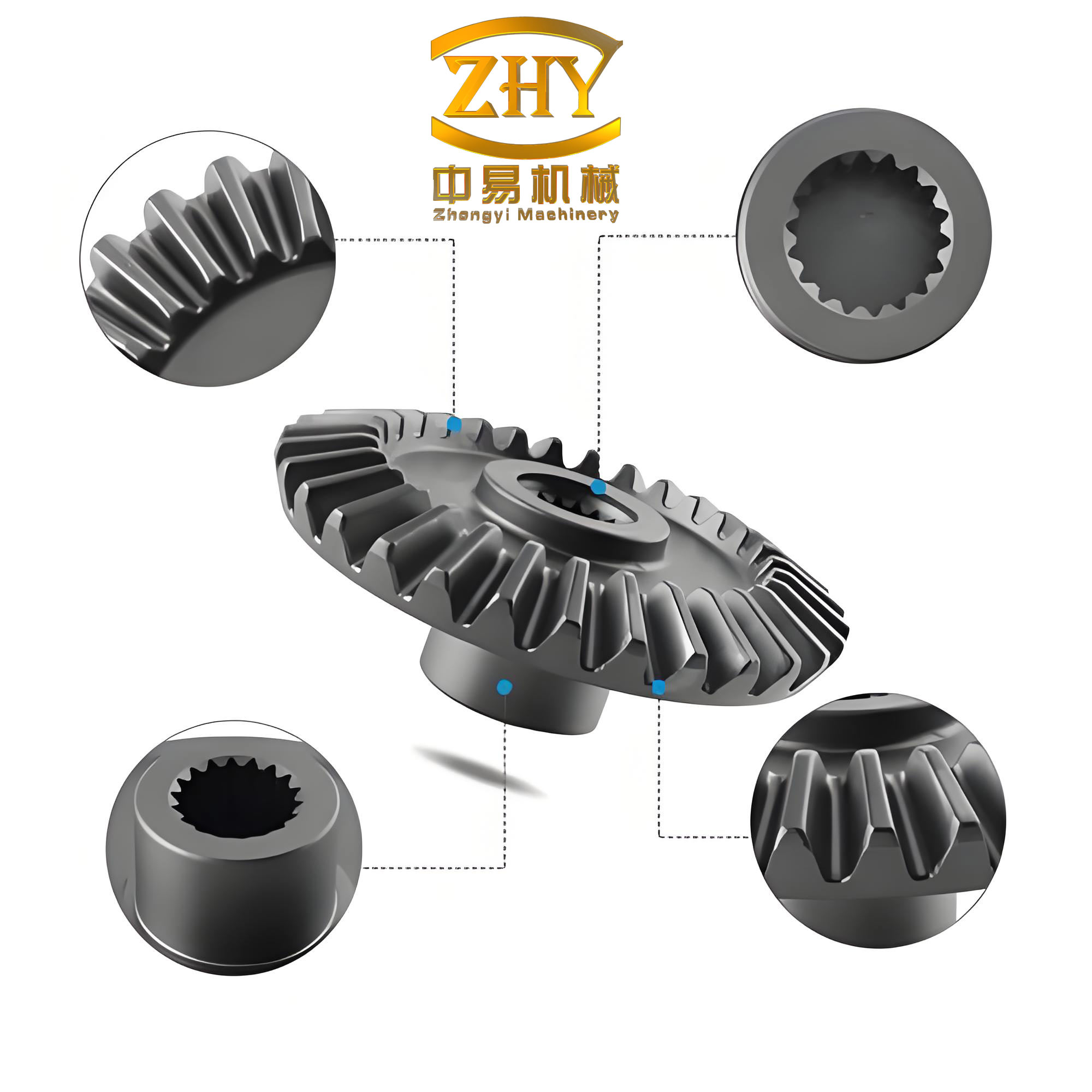
1.4 Start and End Angles of the Tooth Flank Curves
Trimming an involute after it has been generated destroys the parametric link and often makes the tooth space asymmetric. I avoid trimming by controlling the involute parameter directly. The start angle and end angle are computed from the base radius, the root radius, and the tip radius.
For the involute, the start angle depends on whether the root transition curve is present. I write
$$ \phi_{\text{start}} = \operatorname{inv}\alpha_{\text{start}} \times \frac{180^\circ}{\pi} $$
where
$$ \alpha_{\text{start}} = \arccos\left(\frac{r_b}{r_{\text{start}}}\right) $$
The choice of r_start depends on the profile composition:
| Condition | Start radius | Start angle formula |
|---|---|---|
| zv > 17 | Root radius r_f | phi_start = inv( arccos(rb / r_f) ) in degrees |
| zv <= 17 | Connection radius r_c | phi_start = inv( arccos(rb / r_c) ) in degrees |
The end angle is controlled by the tip radius:
$$ \phi_{\text{end}} = \operatorname{inv}\alpha_{\text{end}} \times \frac{180^\circ}{\pi} $$
$$ \alpha_{\text{end}} = \arccos\left(\frac{r_b}{r_a}\right) $$
By using these start and end angles, I generate exactly the needed portion of the involute and the root transition curve. No trimming is required, and the straight bevel gear tooth flank remains symmetric under parameter changes.
2. Parametric Modeling Procedure for the Straight Bevel Gear
I build the straight bevel gear in a feature-based CAD environment. The modeling procedure is driven by expressions, law curves, and datum features. The main steps are:
- Define the basic parameters of the straight bevel gear.
- Compute the derived geometric parameters.
- Define the profile-specific parameters for the involute and root transition curve.
- Create the tooth blank by a revolved sketch.
- Construct the back-cone datum plane and the back-cone datum coordinate system.
- Generate the symmetric involute and root transition curves on the back-cone plane.
- Close the large-end tooth space section with an arc.
- Create a ruled surface between the large-end tooth space and the cone apex.
- Boolean-subtract the ruled surface from the tooth blank.
- Pattern the tooth space around the gear axis.
2.1 Basic Parameters of the Straight Bevel Gear
I set the large-end parameters as the standard values. The basic parameter table contains six independent inputs. These inputs control the main geometry and the tooth form of the straight bevel gear.
| Parameter | Symbol | Example value |
|---|---|---|
| Module | m | 4 mm |
| Pinion tooth number | z1 | 30 |
| Gear tooth number | z2 | 55 |
| Pressure angle | alpha | 20 degrees |
| Addendum coefficient | ha* | 1.0 |
| Clearance coefficient | c* | 0.2 |
2.2 Calculated Parameters of the Straight Bevel Gear
From the basic parameters, I compute the derived parameters. These derived parameters are inserted into the expression list so that the straight bevel gear model updates automatically.
| Parameter | Symbol | Calculation |
|---|---|---|
| Pitch cone angle | delta1, delta2 | delta1 = arctan(z1/z2), delta2 = arctan(z2/z1) |
| Equivalent tooth number | zv1, zv2 | zv1 = z1 / cos(delta1), zv2 = z2 / cos(delta2) |
| Pitch diameter | d | d = m z |
| Tip diameter | da | da = d + 2 ha* m cos(delta) |
| Root diameter | df | df = d – 2 (ha* + c*) m cos(delta) |
| Base radius | rb | rb = d cos(alpha) / 2 |
| Cone distance | R | R = m sqrt(z1^2 + z2^2) / 2 |
| Face width | b | b = R / 3 |
| Addendum | ha | ha = ha* m |
| Dedendum | hf | hf = (ha* + c*) m |
| Addendum angle | theta_a | theta_a = arctan(ha / R) |
| Dedendum angle | theta_f | theta_f = arctan(hf / R) |
| Root cone angle | delta_f | delta_f = delta – theta_f |
| Tip cone angle | delta_a | delta_a = delta + theta_a |
| Tip cone complement | delta_a_complement | delta_a_complement = 180 degrees – theta_f |
2.3 Profile-Specific Parameters
To control the involute and the root transition curve, I add a second group of parameters. These parameters are not independent geometric dimensions; they are mathematical controls for the law curves.
| Parameter | Symbol | Calculation or source |
|---|---|---|
| Involute start angle | phi_start | From start radius, see Section 1.4 |
| Involute end angle | phi_end | From tip radius, see Section 1.4 |
| Involute parameter | u | u = tan(alpha_u) |
| Symmetry angle | gamma | gamma = -90/(4 zv) + inv(alpha) |
| Transition curve parameter | theta | theta = (ha* m – r_c) / (r_p tan(phi)) |
| Connection rotation angle | theta2 | theta2 = inv(alpha) – inv(alpha_c) |
| Cutter corner radius | r_c | Standard cutter value or user input |
2.4 Tooth Blank of the Straight Bevel Gear
I create the tooth blank as a revolved sketch. The sketch contains the pitch cone line, the tip cone line, the root cone line, and the back cone line. The tip cone complement is set to produce equal-clearance bevel gear meshing. I constrain the sketch with expressions so that the straight bevel gear blank changes with the basic parameters.
The tooth blank sketch is driven by the following relations:
$$ d = m z $$
$$ d_a = d + 2 h_a^* m \cos\delta $$
$$ d_f = d – 2(h_a^* + c^*) m \cos\delta $$
$$ R = \frac{m}{2}\sqrt{z_1^2 + z_2^2} $$
$$ b = \frac{R}{3} $$
I revolve the sketch about the straight bevel gear axis. The result is a solid blank with the correct tip cone, root cone, and face width.
2.5 Back-Cone Datum Plane and Datum Coordinate System
The back-cone datum plane and the back-cone datum coordinate system are the most critical features in my parametric method. If they are wrong, the straight bevel gear tooth space will not be positioned correctly. I construct them step by step.
| Step | Operation | Result |
|---|---|---|
| 1 | Make the back-cone line coincide with the pitch cone line and make the gear axis coincide with the cone axis. | The two lines intersect at the cone apex. |
| 2 | Create a sketch plane using the point-and-direction method. Select the cone apex and the back-cone line direction. | Plane I is created perpendicular to the back-cone line. |
| 3 | On Plane I, draw a line through the cone apex along the local Y direction. | The line is constrained to coincide with the back-cone line at the apex. |
| 4 | Create a second plane using the angle-to-plane method. Use Plane I as the plane object and the line from Step 3 as the linear object. | Plane II is the back-cone datum plane. |
| 5 | On Plane II, draw a line that makes an angle gamma1 = -gamma with the back-cone line. | The symmetry line for the involute and transition curve is defined. |
| 6 | Create a third plane using the point-and-direction method. Select the cone apex and the line from Step 5. | Plane III is created for the local X direction. |
| 7 | Insert a datum coordinate system with the symmetry line as the X axis, the line from Step 6 as the Y axis, and the cone apex as the origin. | The back-cone datum coordinate system is complete. |
I use this datum coordinate system as the reference for all law curves. Because the coordinate system is built from the same expressions that drive the straight bevel gear, it updates automatically when the basic parameters change.
2.6 Tooth Space Generation with Ruled Surfaces
After the back-cone datum coordinate system is ready, I generate the large-end tooth space curve. For a straight bevel gear with zv <= 17, I use the involute equation and the root transition curve equation. For a straight bevel gear with zv > 17, I use the involute equation only. I then close the tooth space with an arc at the large end.
The large-end tooth space section is a closed curve. I create a ruled surface between this closed curve and the cone apex. The ruled surface is the cutting tool for the tooth space. The parameters of the ruled surface are:
| Ruled surface parameter | Value or reference |
|---|---|
| Section curve 1 | Cone apex point |
| Section curve 2 | Closed large-end tooth space curve |
| Alignment | Parameter alignment |
| Body type | Solid or sheet depending on CAD kernel |
| Boolean operation | Subtract from tooth blank |
I subtract the ruled surface from the tooth blank. This produces one tooth space. I then add the ruled surface and the subtract feature to a feature group. Using the gear axis as the reference, I pattern the feature group by an angle of 360 degrees divided by z. The result is a complete straight bevel gear with all tooth spaces.
2.7 Solid Verification of the Straight Bevel Gear
After generating the solid, I measure the key dimensions: tip diameter, root diameter, pitch diameter, cone distance, tooth thickness, and tooth space width. I compare the measured values with the theoretical values. The error is typically very small because the law curves are driven by exact equations. The straight bevel gear model remains parametric, and no parent-child relationships are lost.
| Measured quantity | Theoretical value | Typical error |
|---|---|---|
| Tip diameter | da = d + 2 ha* m cos(delta) | < 0.01 mm |
| Root diameter | df = d – 2 (ha* + c*) m cos(delta) | < 0.01 mm |
| Pitch diameter | d = m z | < 0.005 mm |
| Cone distance | R = m sqrt(z1^2 + z2^2) / 2 | < 0.01 mm |
| Tooth thickness | s = m (pi/2 + 2 x tan alpha) | < 0.02 mm |
3. Parametric Realization of the Straight Bevel Gear
I realize full parametric behavior in two ways: by expression-driven update and by spreadsheet-driven update. Both methods keep the straight bevel gear model consistent and avoid manual rework.
3.1 Expression-Driven Update
The basic parameters, calculated parameters, and profile-specific parameters are stored in the expression list. When I change the module, tooth numbers, pressure angle, or coefficients, the following features update automatically:
- The tooth blank sketch.
- The back-cone datum plane.
- The back-cone datum coordinate system.
- The involute start and end angles.
- The symmetry angle.
- The root transition curve parameters.
- The large-end tooth space section.
- The ruled surface cutting tool.
- The circular pattern angle.
Because the symmetric equations are written directly into the law curves, the straight bevel gear tooth space remains symmetric after every update. This is the main advantage of my method over trimming-based approaches.
3.2 Spreadsheet and Part Family Update
For series design and similar design, I use a spreadsheet to manage multiple straight bevel gear sizes. I select the master model, export the basic parameters to the spreadsheet, and add columns for part number, part name, and required gear parameters. When I want to create a new straight bevel gear, I enter the new values in a row, select that row, and execute the create-part command. The CAD system generates a new straight bevel gear model from the master model without rebuilding the feature tree manually.
| Update method | Best use case | Advantage |
|---|---|---|
| Expression list | Single straight bevel gear design | Immediate feedback, full parametric control |
| Spreadsheet | Batch update of one model | Easy editing of many parameters |
| Part family | Series of straight bevel gears | Rapid generation of many models from one master |
3.3 Parameter Table for a Straight Bevel Gear Family
I usually define a parameter table for a straight bevel gear family. The table contains the independent inputs and the derived values that are needed for manufacturing drawings.
| Part number | Module m | Pinion z1 | Gear z2 | Pressure angle alpha | Face width b | Cone distance R |
|---|---|---|---|---|---|---|
| SBG-001 | 3 | 20 | 40 | 20 | 22.36 | 67.08 |
| SBG-002 | 4 | 25 | 50 | 20 | 29.81 | 89.44 |
| SBG-003 | 5 | 18 | 36 | 20 | 33.54 | 100.62 |
| SBG-004 | 6 | 15 | 30 | 20 | 40.25 | 120.75 |
4. Numerical Details and Practical Considerations
I pay attention to several numerical details when I implement the symmetric equations for the straight bevel gear.
4.1 Involute Function and Angle Units
The involute function is defined in radians:
$$ \operatorname{inv}\alpha = \tan\alpha – \alpha $$
When I use the symmetry angle in a CAD expression, I convert it to degrees if the CAD system requires degrees for the mirror line. The conversion is
$$ \gamma_{\text{deg}} = \gamma_{\text{rad}} \times \frac{180^\circ}{\pi} $$
For the start and end angles of the involute, I also convert the involute function to degrees:
$$ \phi_{\text{start,deg}} = \operatorname{inv}\alpha_{\text{start}} \times \frac{180^\circ}{\pi} $$
$$ \phi_{\text{end,deg}} = \operatorname{inv}\alpha_{\text{end}} \times \frac{180^\circ}{\pi} $$
4.2 Bridge Curve at the Connection Point
For a straight bevel gear with zv <= 17, the involute and the root transition curve meet at a connection point. Due to numerical rounding, the two curves may not share exactly the same endpoint. I use a bridge curve to close the gap. The bridge curve is defined by the two endpoints and the tangent directions. I constrain the bridge curve with expressions so that it updates with the straight bevel gear parameters.
4.3 Avoiding Non-Parametric Transforms
I avoid mirror, trim, and transform commands that break the parametric chain. Instead, I use the symmetric equations directly in the law curves. This is the reason the straight bevel gear model remains fully parametric. The symmetric equation is not a post-processing step; it is part of the mathematical definition of the tooth flank.
4.4 Ruled Surface Quality
The ruled surface is generated between the cone apex and the large-end tooth space curve. I use a parameter alignment option to ensure that the surface follows the tooth space curve smoothly. The surface quality is important because it directly affects the solid Boolean operation. If the ruled surface self-intersects, the Boolean subtraction can fail. I therefore check the large-end tooth space curve for self-intersection before creating the ruled surface.
5. Comparison with Conventional Straight Bevel Gear Modeling
Conventional straight bevel gear modeling often uses a combination of involute generation, mirror, trim, and fillet. This approach has several disadvantages. My symmetric-equation method addresses these disadvantages directly.
| Issue in conventional modeling | Effect on straight bevel gear | Symmetric-equation solution |
|---|---|---|
| Asymmetric tooth profile | Meshing simulation and contact analysis become unreliable | Involute and transition curve are mirrored by equations, so symmetry is exact |
| Lost parameters after trim | Model cannot be updated by changing basic parameters | Start and end angles are controlled by expressions, so no trim is needed |
| Root transition curve omitted | Bending stress prediction is inaccurate | Transition curve is generated when zv <= 17 |
| Back-cone datum not parametric | Tooth space moves when gear parameters change | Back-cone datum plane and coordinate system are expression-driven |
| Non-parametric circular pattern | Pattern angle does not update with tooth number | Pattern angle is 360 degrees / z and is fully parametric |
6. Verification of the Straight Bevel Gear Model
I verify the straight bevel gear model by checking the following items:
- The large-end tooth profile is symmetric about the tooth centerline.
- The involute start point lies on the base circle or on the connection circle.
- The involute end point lies on the tip cone.
- The root transition curve connects smoothly to the involute.
- The tooth space closes correctly at the large end.
- The ruled surface does not self-intersect.
- The circular pattern produces exactly z tooth spaces.
- The solid mass properties are consistent with the theoretical volume.
I also perform a parameter sweep. I change the module from 2 mm to 8 mm, the pinion tooth number from 12 to 40, and the gear tooth number from 20 to 80. In every case, the straight bevel gear model updates without failure. The symmetry is preserved, and the root transition curve is generated correctly when the equivalent tooth number is less than or equal to 17.
7. Application Value of the Symmetric-Equation Method
The symmetric-equation method for straight bevel gears has clear application value in series design, similar design, and specialized transmission development. It shortens the design cycle, improves design efficiency, and provides a reliable parametric model for finite element analysis, virtual assembly, and optimization.
| Application area | Benefit of the straight bevel gear model |
|---|---|
| Finite element analysis | Accurate tooth flank and root transition curve improve stress prediction |
| Virtual assembly | Parametric model updates automatically for different gear ratios |
| Optimization | Basic parameters can be driven by an external optimization loop |
| Series design | Part family generates many straight bevel gear sizes from one master |
| Manufacturing drawing | Derived parameters are available in the expression list |
8. Detailed Mathematical Summary
I summarize the main mathematical relations used in the straight bevel gear model. These relations are the core of the parametric definition.
8.1 Equivalent Gear Relations
$$ z_{v1} = \frac{z_1}{\cos \delta_1} $$
$$ z_{v2} = \frac{z_2}{\cos \delta_2} $$
$$ \delta_1 = \arctan\left(\frac{z_1}{z_2}\right) $$
$$ \delta_2 = \arctan\left(\frac{z_2}{z_1}\right) $$
8.2 Involute Relations
$$ x_1 = r_b(\cos u + u \sin u) $$
$$ y_1 = r_b(\sin u – u \cos u) $$
$$ \gamma = -\frac{90^\circ}{4 z_v} + \operatorname{inv}\alpha $$
$$ x_2 = x_1 + \frac{2\sin\gamma\,(y_1 – x_1\sin\gamma)}{1+\sin^2\gamma} $$
$$ y_2 = y_1 – \frac{2(y_1 – x_1\sin\gamma)}{1+\sin^2\gamma} $$
8.3 Root Transition Relations
$$ x_0 = r_c \cos\phi $$
$$ y_0 = r_c(1-\sin\phi) – h_a^* m $$
$$ \theta = \frac{h_a^* m – r_c}{r_p \tan\phi} $$
$$ x_t = x_0\cos\theta + y_0\sin\theta + r_c(\theta\sin\theta + \cos\theta) $$
$$ y_t = x_0\sin\theta – y_0\cos\theta + r_c(\theta\cos\theta – \sin\theta) $$
$$ \theta_2 = \operatorname{inv}\alpha – \operatorname{inv}\alpha_c $$
$$ x_{t2} = x_t + \frac{2\sin\gamma\,(y_t – x_t\sin\gamma)}{1+\sin^2\gamma} $$
$$ y_{t2} = y_t – \frac{2(y_t – x_t\sin\gamma)}{1+\sin^2\gamma} $$
8.4 Start and End Angle Relations
$$ \phi_{\text{start}} = \operatorname{inv}\left(\arccos\left(\frac{r_b}{r_{\text{start}}}\right)\right) \times \frac{180^\circ}{\pi} $$
$$ \phi_{\text{end}} = \operatorname{inv}\left(\arccos\left(\frac{r_b}{r_a}\right)\right) \times \frac{180^\circ}{\pi} $$
9. Practical Implementation Steps in a Feature-Based CAD System
I implement the straight bevel gear model with the following exact sequence. This sequence can be adapted to any feature-based CAD system that supports expressions, law curves, datum planes, datum coordinate systems, ruled surfaces, and circular patterns.
- Create the basic parameter expressions: m, z1, z2, alpha, ha*, c*.
- Create the calculated parameter expressions: delta1, delta2, zv1, zv2, d1, d2, da1, da2, df1, df2, rb1, rb2, R, b, ha, hf, theta_a, theta_f, delta_f, delta_a.
- Create the profile-specific expressions: gamma1, gamma2, phi_start1, phi_start2, phi_end1, phi_end2, u, theta, theta2.
- Sketch the tooth blank on the front plane. Use the calculated expressions to drive the pitch cone line, tip cone line, root cone line, and back cone line.
- Revolve the sketch around the gear axis to create the solid tooth blank.
- Construct the back-cone datum plane using the point-and-direction method and the angle-to-plane method.
- Construct the back-cone datum coordinate system using the symmetry line and the local Y direction.
- Create the involute law curve on the back-cone datum plane. Use the symmetric equation to generate both flanks.
- If zv <= 17, create the root transition law curve. Use the connection rotation and the symmetric equation to generate both flanks.
- Close the large-end tooth space section with an arc.
- Create a ruled surface between the cone apex and the closed tooth space section.
- Subtract the ruled surface from the tooth blank.
- Group the ruled surface and the subtract feature.
- Pattern the group around the gear axis by 360 degrees / z.
- Verify the solid and measure the key dimensions.
10. Conclusion
I have presented a symmetric-equation method for the parametric modeling of involute straight bevel gears. The method is based on the back-cone equivalent gear, the boundary equivalent tooth number, symmetric equations for the involute and the root transition curve, exact start and end angles, a parametric back-cone datum plane and coordinate system, and a ruled-surface cutting strategy. The straight bevel gear model remains fully parametric, symmetric, and robust under parameter changes.
The method avoids the common problems of asymmetric tooth profiles, lost parameters, and non-parametric trimming. It is practical and operable in a feature-based CAD environment. I have verified the method with multiple parameter sets and confirmed that the geometric dimensions match the theoretical values with very small error. The straight bevel gear model can be updated by expressions, spreadsheets, or part families, making it suitable for series design, similar design, and specialized transmission development.
In future work, I will extend the symmetric-equation approach to spiral bevel gears and hypoid gears, where the tooth flank is generated by a more complex cutting motion. I will also integrate the straight bevel gear model with finite element analysis and optimization workflows to further shorten the design cycle.