
I present a first-person account of a computational study on the time-varying meshing stiffness of herringbone gear pairs, with a framework that can also be adapted to miter gear and other high-load gear transmissions. The work combines exact tooth-surface generation, finite element contact analysis, analytical contact-line modeling, and parametric studies of errors and modifications. Throughout the study, I treat meshing stiffness as a central internal excitation parameter because it controls dynamic contact force, transmission error, vibration, noise, and fatigue life. The term miter gear appears repeatedly here as a reference point for generalized gear contact and stiffness modeling, although the specific numerical examples are for a double-helical herringbone gear pair. The same computational philosophy—geometry generation, contact solution, deformation extraction, and stiffness synthesis—can be transferred to miter gear applications where load sharing and contact-line effects are important.
1. Research Context and Motivation
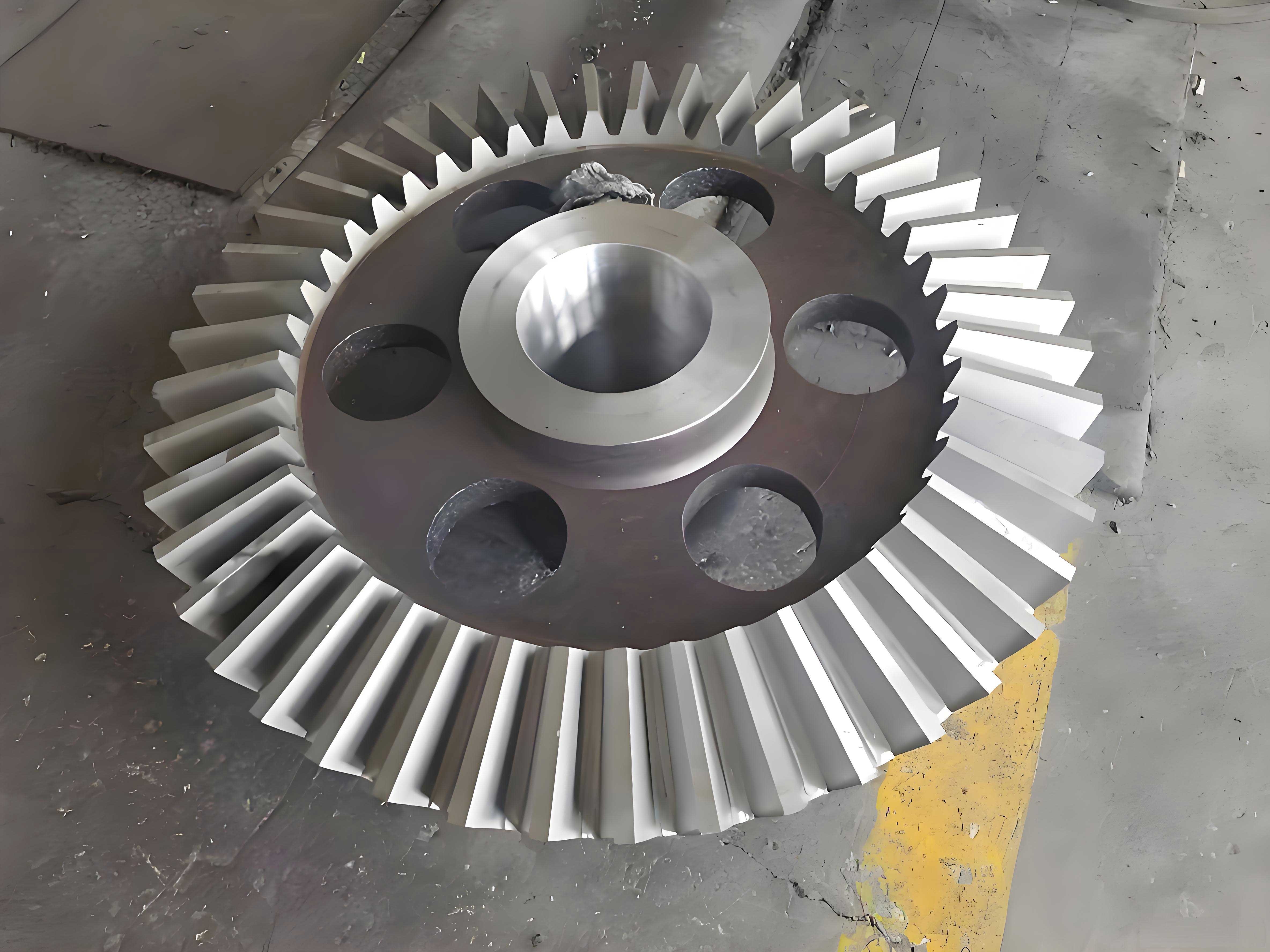
I began with the observation that herringbone gears offer high contact ratio, low axial force, high load capacity, and smooth transmission. These properties make them attractive for energy equipment, large ships, high-speed aerospace drives, and heavy-duty reducers. A miter gear, by contrast, is often used for intersecting-axis motion, but the broader family of precision gear drives—including miter gear systems—also benefits from accurate stiffness prediction because load distribution and dynamic response depend on contact compliance. My objective was therefore to establish a robust method for computing the meshing stiffness of a herringbone gear pair and then to quantify how assembly errors, alignment errors, profile modification, and lead crowning change that stiffness. The same questions arise in miter gear design when contact patterns shift under load or misalignment.
Meshing stiffness is not a single constant. It varies with rotation angle, contact position, number of engaged teeth, load level, and manufacturing or assembly deviation. For a gear pair, I distinguish three quantities:
- single-tooth stiffness, which describes one tooth of one gear under load;
- single-pair meshing stiffness, which combines the two mating teeth in series;
- total meshing stiffness, which combines all simultaneously engaged tooth pairs in parallel.
The basic definition I used is
$$K_n=\frac{F_n}{u_n}$$
where \(F_n\) is the normal contact force on the tooth surface and \(u_n\) is the comprehensive elastic deformation. The comprehensive deformation includes Hertzian contact deformation \(u_H\) and tooth bending deformation \(u_b\). I did not include shaft, bearing, or housing compliance in the present numerical model, so
$$u_n=u_H+u_b.$$
For a single meshing pair, the two gear teeth act in series. If the driving gear stiffness is \(K_1\) and the driven gear stiffness is \(K_2\), then
$$K_{\mathrm{pair}}=\frac{K_1K_2}{K_1+K_2}.$$
For multiple engaged pairs, the total stiffness is the parallel sum:
$$K_{\mathrm{total}}=\sum_{i=1}^{n}K_i.$$
These equations form the backbone of the entire study. I used them for standard gears, for gears with errors, and for gears with modifications. I also used them to compare finite element results with analytical predictions. A miter gear transmission can be analyzed with analogous series and parallel combinations once its contact force and deformation are known.
2. Geometry and Finite Element Model
I derived the tooth profile using the generating principle of a rack cutter. The rack and gear blank move relative to each other, and the envelope of the cutter edge produces the involute profile and the root fillet. This approach gives a precise geometric description that is more reliable than approximating the involute with simple arcs. The coordinate transformation between the rack coordinate system and the gear blank coordinate system can be written as
$$
\begin{bmatrix}
x_2\\
y_2\\
1
\end{bmatrix}
=
M_{21}
\begin{bmatrix}
x_1\\
y_1\\
1
\end{bmatrix}
$$
with
$$
M_{21}=
\begin{bmatrix}
\cos\varphi & \sin\varphi & r\sin\varphi+r\varphi\cos\varphi\\
-\sin\varphi & \cos\varphi & r\cos\varphi-r\varphi\sin\varphi\\
0 & 0 & 1
\end{bmatrix}.
$$
Here \(r\) is the pitch radius of the gear blank, and \(\varphi\) is the rotation angle of the gear blank. The general profile equation becomes
$$
\begin{aligned}
x_2 &= r\cos\varphi + x_1\cos\varphi + y_1\sin\varphi – r\varphi\sin\varphi,\\
y_2 &= r\sin\varphi – x_1\sin\varphi + y_1\cos\varphi – r\varphi\cos\varphi.
\end{aligned}
$$
For the root fillet, the cutter tip radius generates a transition curve. If \((x_c,y_c)\) is the center of the cutter tip arc and \(\rho\) is the tip radius, then a point on the fillet in the cutter coordinate system is
$$
\begin{aligned}
x_1 &= x_c+\rho\cos\gamma,\\
y_1 &= y_c-\rho\sin\gamma,
\end{aligned}
$$
where
$$\gamma=\arctan\left(\frac{r-y_c}{x_c}\right).$$
Substituting these expressions into the coordinate transformation yields the root fillet equation. For the involute portion, the straight edge of the rack produces
$$
\begin{aligned}
x_1 &= r\varphi – (y_0-r\varphi)\sin\alpha\cos\alpha,\\
y_1 &= r\varphi\sin^2\alpha – y_0,
\end{aligned}
$$
where \(\alpha\) is the pressure angle and \(y_0\) is the position of the straight edge. The resulting involute equation is
$$
\begin{aligned}
x_2 &= \frac{1}{2}r\sin(2\varphi) – r\varphi\cos^2\varphi + y_0\sin\varphi,\\
y_2 &= \frac{1}{2}r\sin(2\varphi) – r\varphi\sin\varphi\cos\varphi – y_0\cos\varphi.
\end{aligned}
$$
For the helical tooth surface, I extended the transverse profile along a helix. A point on the helical surface is described by
$$
\begin{aligned}
X &= R\cos\left(\frac{B}{r}\tan\beta\,t\right),\\
Y &= R\sin\left(\frac{B}{r}\tan\beta\,t\right),\\
Z &= Bt,\qquad 0\le t\le 1,
\end{aligned}
$$
where \(R=\sqrt{x_2^2+y_2^2}\), \(B\) is the face width, and \(\beta\) is the helix angle. For a herringbone gear, which is effectively two opposite-hand helical gears joined together, the surface is mirrored about the mid-plane. If the central relief groove width is \(B_w\), the herringbone surface can be written as
$$
\begin{aligned}
X &= R\cos\left(\frac{B}{r}\tan\beta\,t\right),\\
Y &= R\sin\left(\frac{B}{r}\tan\beta\,t\right),\\
Z &= \pm\left(\frac{B}{2}+B_w+Bt\right),\qquad 0\le t\le 1.
\end{aligned}
$$
I used these equations in a numerical script to generate discrete tooth-surface points. The points were imported into a three-dimensional modeling environment, where I fitted curves and surfaces to produce a smooth herringbone gear geometry. The basic parameters of the gear pair are listed in Table 1.
| Parameter | Driving gear | Driven gear |
|---|---|---|
| Number of teeth \(z\) | 34 | 31 |
| Normal module \(m_n\) (mm) | 6 | 6 |
| Normal pressure angle \(\alpha_n\) (deg) | 25 | 25 |
| Helix angle \(\beta\) (deg) | 35.9891 | 35.9891 |
| Face width per helix \(b_1\) (mm) | 180 | 180 |
| Relief groove width \(b_2\) (mm) | 24 | 24 |
| Relief groove depth \(d\) (mm) | 5.5 | 4 |
| Torque \(T\) (N·m) | 9545 | 9545 |
For the finite element model, I divided the geometry into several sweepable regions. The tooth surface was partitioned so that structured hexahedral meshes could be generated. I used linear reduced-integration elements because they are robust for contact problems and reduce shear locking. The material properties are given in Table 2.
| Property | Value |
|---|---|
| Material | 45 steel equivalent |
| Elastic modulus \(E\) (GPa) | 210 |
| Poisson ratio \(\mu\) | 0.3 |
| Density \(\rho\) (kg/m³) | 7.8 |
| Friction coefficient at contact | 0.06 |
I created a reference point on the rotation axis of each gear and coupled it to the inner surface of the gear body. This allowed me to apply torque and rotation while avoiding unphysical rigid-body motion. For static analysis, I used a general static step and applied a prescribed rotation to one gear and a torque to the other. For dynamic analysis, I used an explicit dynamic step. To improve convergence, I applied speed and torque in separate steps with smooth amplitude curves. Contact pairs were defined on the tooth flanks, and the friction coefficient was set to 0.06 to represent the sliding contact condition.
3. Static and Dynamic Contact Analysis
I first performed a static loading analysis. The load case is summarized in Table 3. The static contact force distribution for a complete meshing cycle showed that the normal contact force on a single tooth increases gradually, reaches a maximum near the midpoint of engagement, and then decreases. This parabolic-like trend is consistent with the change in contact position and the changing number of engaged teeth. Adjacent tooth pairs showed nearly identical contact force histories, which indicates good transmission continuity.
| Case | Rotation angle (rad) | Torque (N·m) |
|---|---|---|
| Static | 1.5 | 9545 |
The contact ratio was obtained from the contact-force history. If one tooth remains in contact for a duration \(\Delta T\), and the adjacent tooth enters contact after a time interval \(\Delta t\), then
$$\varepsilon=\frac{\Delta T}{\Delta t}.$$
From the finite element results, I found \(\Delta T=0.76\) s and \(\Delta t=0.19\) s, giving \(\varepsilon=4.0\). This high contact ratio is one reason why herringbone gears transmit load smoothly and why the total meshing stiffness is high.
Under the static load, the maximum contact stress was 364.9 MPa, and the maximum bending stress was 120.6 MPa. The contact stress at the beginning of engagement was 484.9 MPa, while at the end of engagement it was 535.8 MPa. These values indicate that the meshing-in and meshing-out positions experience higher local stress than the central region. Table 4 summarizes the static stress results.
| Quantity | Value |
|---|---|
| Maximum contact stress | 364.9 MPa |
| Maximum bending stress | 120.6 MPa |
| Contact stress at meshing-in | 484.9 MPa |
| Contact stress at meshing-out | 535.8 MPa |
I then performed dynamic contact analyses at four rotational speeds. The load cases are listed in Table 5. I kept the torque constant and varied the speed from 1000 to 10000 rpm. This allowed me to isolate speed effects and to observe how a miter gear-like contact pattern would change under high-speed operation, even though the present geometry is a herringbone gear.
| Case | Speed (r/min) | Torque (N·m) |
|---|---|---|
| Case 2 | 1000 | 9545 |
| Case 3 | 5000 | 9545 |
| Case 4 | 8000 | 9545 |
| Case 5 | 10000 | 9545 |
In the dynamic analysis, I observed that the driving and driven gears reached steady speed after a short transient. At 1000 rpm, the speed was stable. At 5000 rpm, the driving gear speed was stable while the driven gear speed showed slight fluctuation. At 8000 rpm and 10000 rpm, the driven gear speed fluctuated more strongly, indicating that high-speed operation increases dynamic coupling and contact loss. The time to reach steady speed decreased as the rotational speed increased: approximately 0.018 s at 1000 rpm, 0.0036 s at 5000 rpm, 0.0022 s at 8000 rpm, and 0.002 s at 10000 rpm.
The contact force histories showed a clear acceleration stage and a stable running stage. During the initial engagement, the contact force oscillated strongly because of impacts. At higher speeds, the oscillation amplitude increased, and the contact force became larger under the same torque. At 8000 rpm and 10000 rpm, I observed intervals of zero contact force on the normal flanks, followed by contact on the opposite flanks. This means the gear pair experienced contact loss and back-side contact. The observed sequence was normal contact, loss of contact, back-side contact, and return to normal contact. This behavior is important for miter gear and other high-speed gear systems because it can cause noise, wear, and fatigue.
The contact area followed the same trend as the contact force. Under the same torque, the contact area increased with speed. At the highest speeds, the contact area also showed zero intervals, confirming the intermittent contact behavior. The maximum contact stress and maximum bending stress increased with speed, as shown in Table 6. The maximum contact stress location was near the middle of the tooth width, and the maximum bending stress occurred below the contact region.
| Case | Speed (r/min) | Maximum contact stress (MPa) | Maximum bending stress (MPa) |
|---|---|---|---|
| Case 2 | 1000 | 877.2 | 289.3 |
| Case 3 | 5000 | 2800.0 | 1574.6 |
| Case 4 | 8000 | 5203.0 | 4803.0 |
| Case 5 | 10000 | 6829.6 | 5468.9 |
The dynamic results show that lower speeds produce smoother transmission. At high speeds, impact and back-side contact become significant. The contact and bending stresses rise sharply, which can lead to wear and surface damage. These findings motivated the subsequent stiffness calculations and the studies of errors and modifications.
4. Standard Meshing Stiffness Calculation
I calculated the meshing stiffness of the standard herringbone gear pair using both finite element analysis and an analytical method. The finite element method was based on the normal contact force and comprehensive deformation extracted from the contact solution. The analytical method was based on the instantaneous total contact line length and the unit contact-line stiffness.
4.1 Finite Element Stiffness Calculation
For each meshing position, I extracted the normal contact force \(F_n\) and the average elastic deformation \(u_n\) over the contact region. The single-tooth stiffness of the driving gear was \(K_1=F_n/u_{n1}\), and the single-tooth stiffness of the driven gear was \(K_2=F_n/u_{n2}\). The single-pair meshing stiffness was then obtained from the series combination in Eq. (3). To capture the time-varying nature, I divided one complete meshing cycle into 25 positions. Each position corresponded to a rotation increment of 0.03 rad. The calculated stiffness values for selected positions are listed in Table 7.
| Driving gear rotation (rad) | Driving gear stiffness (N/m) | Driven gear stiffness (N/m) |
|---|---|---|
| 0.03 | 1.898686×10^8 | 3.067052×10^8 |
| 0.06 | 7.367521×10^8 | 6.091630×10^8 |
| 0.09 | 1.212667×10^9 | 9.290257×10^8 |
| 0.12 | 1.675959×10^9 | 1.363793×10^9 |
| 0.15 | 2.198675×10^9 | 1.875465×10^9 |
| 0.18 | 2.497343×10^9 | 2.449099×10^9 |
| 0.21 | 2.687129×10^9 | 3.112956×10^9 |
| 0.24 | 2.900461×10^9 | 3.559245×10^9 |
| 0.27 | 3.037737×10^9 | 3.750572×10^9 |
| 0.30 | 3.131559×10^9 | 3.894012×10^9 |
| 0.33 | 3.210415×10^9 | 3.864422×10^9 |
| 0.36 | 3.213005×10^9 | 3.860768×10^9 |
| 0.39 | 3.219164×10^9 | 3.909906×10^9 |
| 0.42 | 3.242201×10^9 | 3.875142×10^9 |
| 0.45 | 3.238331×10^9 | 3.813841×10^9 |
| 0.48 | 3.165176×10^9 | 3.759140×10^9 |
| 0.51 | 3.071321×10^9 | 3.540088×10^9 |
| 0.54 | 2.849351×10^9 | 3.301845×10^9 |
| 0.57 | 2.296435×10^9 | 3.046531×10^9 |
| 0.60 | 1.851348×10^9 | 2.734256×10^9 |
| 0.63 | 1.396123×10^9 | 2.267925×10^9 |
| 0.66 | 1.015858×10^9 | 1.839452×10^9 |
| 0.69 | 7.008340×10^8 | 1.175099×10^9 |
| 0.72 | 4.466770×10^8 | 5.827601×10^8 |
| 0.75 | 9.361600×10^7 | 3.976300×10^7 |
From these values, I observed that the driving gear stiffness is relatively high at the beginning of engagement and decreases toward the end. The driven gear stiffness shows the opposite trend: it is low at the beginning and high near the middle and end. The single-pair stiffness was obtained from Eq. (3). To construct the total stiffness, I shifted the single-pair stiffness curve by multiples of the angular pitch and summed the contributions from all engaged pairs. The angular shift is
$$\Delta\alpha=\frac{\Phi}{\varepsilon},$$
where \(\Phi\) is the rotation angle in one meshing cycle. Because the contact ratio was 4.0, four tooth pairs contributed simultaneously over much of the cycle. The resulting total stiffness curve is smoother than the single-pair curve and has a higher mean value. This is a key advantage of a herringbone gear and would also be valuable in a miter gear train if the contact ratio can be made sufficiently high.
4.2 Analytical Stiffness Calculation
For the analytical method, I calculated the instantaneous total contact line length on the meshing plane. The total stiffness was then
$$K(t)=2c_\gamma L(t),$$
where \(c_\gamma\) is the stiffness per unit contact line length and \(L(t)\) is the instantaneous contact line length of one helical half. The factor of two accounts for the two opposite-hand halves of the herringbone gear. The contact line length depends on the transverse contact ratio \(\varepsilon_\alpha\) and the overlap contact ratio \(\varepsilon_\beta\). I considered two cases: \(\varepsilon_\alpha<\varepsilon_\beta\) and \(\varepsilon_\alpha>\varepsilon_\beta\).
For a single tooth, the contact line length \(l_1(t)\) is piecewise. When \(\varepsilon_\alpha<\varepsilon_\beta\),
$$
l_1(t)=
\begin{cases}
\dfrac{p_{bt}t}{T_m\sin\beta}, & 0<t<\varepsilon_\alpha $$="" &="" 0,="" <p="" \dfrac{p_{bt}(\varepsilon_\gamma="" \dfrac{p_{bt}}{\sin\beta},="" \end{cases}="" \varepsilon_\alpha="" \varepsilon_\beta="" \varepsilon_\gamma="" t_m,\\[6pt]="" t_m-t)}{t_m\sin\beta},="" t_m<t<(m+1)t_m,="" t_m<t<\varepsilon_\beta="" t_m<twhere \(p_{bt}\) is the base pitch, \(T_m\) is the meshing period, \(\varepsilon_\gamma\) is the total contact ratio, and \(M\) is the largest integer less than \(\varepsilon_\gamma\). When \(\varepsilon_\alpha>\varepsilon_\beta\), the order of the plateaus changes, but the Fourier representation of the contact line length remains the same. I expressed \(l_1(t)\) as a Fourier series:
$$
l_1(t)=\frac{a_0}{2}+\sum_{n=1}^{\infty}\left[a_n\cos\left(\frac{2\pi n t}{(M+1)T_m}\right)+b_n\sin\left(\frac{2\pi n t}{(M+1)T_m}\right)\right],
$$
with coefficients
$$
\begin{aligned}
a_0 &= \frac{2p_{bt}}{(M+1)\sin\beta},\\
a_n &= \frac{2p_{bt}}{\pi n\sin\beta}\left(\cos\frac{2\pi n\varepsilon_\alpha}{M+1}+\cos\frac{2\pi n\varepsilon_\beta}{M+1}-\cos\frac{2\pi n\varepsilon_\gamma}{M+1}-1\right),\\
b_n &= \frac{2p_{bt}}{\pi n\sin\beta}\left(\sin\frac{2\pi n\varepsilon_\alpha}{M+1}+\sin\frac{2\pi n\varepsilon_\beta}{M+1}-\sin\frac{2\pi n\varepsilon_\gamma}{M+1}\right).
\end{aligned}
$$
The total contact line length for all teeth is the sum of shifted single-tooth contact lines. If the shift is \(T_m\), then
$$L(t)=\sum_{i=1}^{M+1}l_1(t+iT_m).$$
After simplification, the total contact line length can be written as
$$
L(t)=\frac{p_{bt}}{\sin\beta}\left[\varepsilon_\alpha+\sum_{k=1}^{\infty}\left(a_k\cos(2\pi k\omega_m t)+b_k\sin(2\pi k\omega_m t)\right)\right],
$$
where \(k=n/(M+1)\) is an integer, and \(\omega_m=1/T_m\). The coefficients are
$$
\begin{aligned}
a_k &= \frac{1}{2\pi k}\left(\cos 2\pi k\varepsilon_\alpha+\cos 2\pi k\varepsilon_\beta-\cos 2\pi k\varepsilon_\gamma-1\right),\\
b_k &= \frac{1}{2\pi k}\left(\sin 2\pi k\varepsilon_\alpha+\sin 2\pi k\varepsilon_\beta-\sin 2\pi k\varepsilon_\gamma\right).
\end{aligned}
$$
The unit contact-line stiffness \(c_\gamma\) was calculated according to the ISO approach. The single-pair stiffness is
$$c’=\frac{1}{q},$$
where \(q\) is the flexibility per unit face width in mm·μm/N. The flexibility \(q\) is obtained from
$$
q=C_1+C_2x_1+C_3x_2+C_4x_1^2+C_5x_1x_2+C_6x_2^2+C_7x_1^3+C_8x_1^2x_2+C_9x_1x_2^2,
$$
with the coefficients listed in Table 8. Here \(x_1\) and \(x_2\) are the profile shift coefficients, and the equivalent tooth numbers are used where required. The corrected single-pair stiffness is
$$c’_{\mathrm{th}}=c’C_MC_RC_B\cos\beta,$$
where \(C_M=0.8\), \(C_R=1\), and \(C_B=1\) for the present case. The mesh stiffness per unit contact line is then
$$c_\gamma=(0.75\varepsilon_\alpha+0.25)c’.$$
Using these equations, I obtained the analytical total stiffness. The comparison with the finite element method is given in Table 9. The maximum single-pair stiffness from the analytical method was \(1.650\times10^9\) N/m, while the finite element method gave \(1.765\times10^9\) N/m. The maximum total stiffness from the analytical method was \(4.660\times10^9\) N/m, while the finite element method gave \(4.778\times10^9\) N/m. The differences were about 7.0% for the single-pair stiffness and about 2.0% for the total stiffness. This agreement validated the finite element stiffness calculation and gave me confidence to use it for error and modification studies.
| Coefficient | Value |
|---|---|
| \(C_1\) | 0.04723 |
| \(C_2\) | 0.15551 |
| \(C_3\) | 0.25791 |
| \(C_4\) | -0.00635 |
| \(C_5\) | -0.11654 |
| \(C_6\) | -0.00193 |
| \(C_7\) | -0.24188 |
| \(C_8\) | 0.00529 |
| \(C_9\) | 0.00182 |
| Method | Maximum single-pair stiffness (N/m) | Maximum total stiffness (N/m) |
|---|---|---|
| Analytical | \(1.650\times10^9\) | \(4.660\times10^9\) |
| Finite element | \(1.765\times10^9\) | \(4.778\times10^9\) |
| Difference | \(0.115\times10^9\) (7.0%) | \(0.118\times10^9\) (2.0%) |
The small discrepancy is mainly due to the finite element model omitting part of the gear body and using rigid coupling at the inner surface. The analytical method assumes a perfect contact line and does not include the exact tooth-root flexibility distribution. Even so, the two methods are close enough for engineering predictions. The finite element method is especially useful when errors and modifications break the symmetry of the contact pattern.
5. Effects of Errors on Meshing Stiffness
I next studied how errors change the meshing stiffness. Two error families were considered: assembly errors and center alignment errors. Assembly errors describe shaft misalignment. Center alignment errors describe the mismatch between the left-hand and right-hand tooth traces of a herringbone gear. Both types of error are important for miter gear and herringbone gear systems because they cause uneven load distribution along the face width.
5.1 Assembly Errors
I considered two components of shaft parallel misalignment: the misalignment in the plane of the axes, \(\Delta f_x\), and the misalignment in the perpendicular plane, \(\Delta f_y\). According to gear design practice, these two components are related by
$$\Delta f_x=2\Delta f_y.$$
For a grade 7 assembly, I selected \(\Delta f_y=24\) μm and 48 μm, which correspond to \(\Delta f_x=48\) μm and 96 μm. The error cases are listed in Table 10.
| Case | \(\Delta f_x\) (μm) | \(\Delta f_y\) (μm) | Description |
|---|---|---|---|
| A0 | 0 | 0 | No error |
| A1 | 48 | 0 | Axial-plane misalignment |
| A2 | 96 | 0 | Larger axial-plane misalignment |
| A3 | 0 | 24 | Perpendicular-plane misalignment |
| A4 | 0 | 48 | Larger perpendicular-plane misalignment |
For the axial-plane misalignment \(\Delta f_x\), I found that the single-pair and total meshing stiffness both decreased as the error increased. The contact stress contours showed that the load was no longer symmetric between the two halves of the herringbone gear. At \(\Delta f_x=48\) μm, one end carried more load than the other. At \(\Delta f_x=96\) μm, one end carried almost no load. The contact force on the lightly loaded side became nearly zero. This unequal load sharing reduces the effective stiffness because the total load is carried by a smaller contact area and fewer active tooth portions.
For the perpendicular-plane misalignment \(\Delta f_y\), the trend was similar. The stiffness decreased with increasing error. The contact stress contours showed uneven load distribution across the face width. The load on one side was significantly lower than on the other side. When I compared the two misalignment directions, I found that the perpendicular-plane error \(\Delta f_y\) had a stronger effect on the meshing stiffness than the axial-plane error \(\Delta f_x\) of the same nominal magnitude. This is an important result for miter gear and herringbone gear installation because it means that controlling the perpendicular-plane alignment is especially critical.
Table 11 summarizes the qualitative effect of assembly errors on stiffness and load sharing.
| Error type | Stiffness trend | Load sharing | Contact pattern |
|---|---|---|---|
| No error | Reference | Symmetric | Uniform along face width |
| Axial-plane misalignment | Decreases with error | Uneven | One end overloaded |
| Perpendicular-plane misalignment | Decreases more strongly | Uneven | Strong edge loading |
5.2 Center Alignment Error
For a herringbone gear, center alignment error describes the mismatch between the left-hand and right-hand helical tooth traces. I modeled the driven gear with a center alignment error \(\delta\), while the driving gear was assumed perfect. I considered \(\delta=20\) μm and 30 μm. The error cases are listed in Table 12.
| Case | \(\delta\) (μm) | Description |
|---|---|---|
| C0 | 0 | No center alignment error |
| C1 | 20 | Small center alignment error |
| C2 | 30 | Larger center alignment error |
The center alignment error also caused uneven load distribution between the two halves of the herringbone gear. As the error increased, the single-pair and total meshing stiffness decreased. The contact stress contours showed that one half of the gear carried more load than the other. The contact force on one side became smaller than on the other side. This behavior is similar to the assembly misalignment case, but the physical cause is different: the left and right tooth traces are not perfectly aligned, so the two halves do not share the load equally.
The stiffness reduction caused by center alignment error is important for manufacturing quality control. If the center alignment error is too large, the gear may operate with only one half carrying most of the load. This can lead to premature wear, higher local stress, and reduced effective stiffness. The same concern applies to a miter gear pair when the two members are not properly aligned.
6. Effects of Modifications on Meshing Stiffness
I also studied two modification types: profile modification and lead crowning. The purpose of these modifications is to reduce meshing impact, improve load distribution, and increase transmission smoothness. However, modification removes material, so it can also reduce stiffness if the modification amount is too large. My goal was to find the trend and to identify the range where modification is beneficial.
6.1 Profile Modification
Profile modification was applied near the tooth tip and root. I used a parabolic modification curve, also known as a Walker curve:
$$\Delta=\Delta_{\max}\left(\frac{x}{h}\right)^n,$$
where \(\Delta_{\max}\) is the maximum modification amount, \(h\) is the modification height, \(x\) is the coordinate measured from the modification start point along the line of action, and \(n\) is the curve exponent. I used \(n=2\) to obtain a smooth parabolic curve. The modification height was 3 mm. I considered \(\Delta_{\max}=5\) μm, 10 μm, and 15 μm. The cases are listed in Table 13.
| Case | \(\Delta_{\max}\) (μm) | Modification height \(h\) (mm) | Curve exponent \(n\) |
|---|---|---|---|
| P0 | 0 | 3 | 2 |
| P1 | 5 | 3 | 2 |
| P2 | 10 | 3 | 2 |
| P3 | 15 | 3 | 2 |
The finite element results showed that the meshing-in and meshing-out contact stresses decreased significantly after profile modification. For the unmodified gear, the contact stress at meshing-in was 484.9 MPa and at meshing-out was 535.8 MPa. With \(\Delta_{\max}=5\) μm, these values dropped to 368.0 MPa and 329.3 MPa. With \(\Delta_{\max}=10\) μm, they dropped to 280.3 MPa and 308.9 MPa. With \(\Delta_{\max}=15\) μm, they dropped to 255.2 MPa and 261.8 MPa. The reduction at meshing-out reached about 51.1%. This means that profile modification effectively suppresses meshing impact.
The maximum contact stress did not change much. For the unmodified gear it was 364.9 MPa, and for the modified gears it ranged from 345.3 MPa to 359.3 MPa. The contact area became shorter in length and slightly wider, and the edge stress concentration was reduced.
For stiffness, I found a non-monotonic trend. When the modification amount was small, the single-pair and total meshing stiffness increased compared with the unmodified gear. This is because the modification reduced the impact and improved the contact load distribution. However, as the modification amount increased, the stiffness increase diminished. When \(\Delta_{\max}=15\) μm, the stiffness became lower than that of the unmodified gear. The reason is that too much material was removed, so the effective load-carrying cross-section was reduced.
Table 14 summarizes the profile modification results.
| \(\Delta_{\max}\) (μm) | Maximum contact stress (MPa) | Meshing-in stress (MPa) | Meshing-out stress (MPa) | Stiffness trend |
|---|---|---|---|---|
| 0 | 364.9 | 484.9 | 535.8 | Reference |
| 5 | 345.3 | 368.0 | 329.3 | Slightly higher |
| 10 | 346.9 | 280.3 | 308.9 | Higher, but less than small modification |
| 15 | 359.3 | 255.2 | 261.8 | Lower than unmodified |
6.2 Lead Crowning
Lead crowning was applied along the face width to improve the load distribution. I used a parabolic crowning curve. According to the ISO recommended formula, the crowning amount is related to the elastic deformation and helix deviation. For high-precision, high-reliability gears, the crowning amount is usually taken as 60% to 70% of the calculated value, giving a range of about 10 μm to 25 μm. I considered \(C_c=10\) μm, 15 μm, and 20 μm. The cases are listed in Table 15.
| Case | \(C_c\) (μm) | Crowning type |
|---|---|---|
| L0 | 0 | No crowning |
| L1 | 10 | Small crowning |
| L2 | 15 | Medium crowning |
| L3 | 20 | Larger crowning |
The contact stress results showed that lead crowning improved the load distribution along the contact line. The maximum contact stress decreased, and the edge stress concentration was reduced. The contact area remained similar to the unmodified case, but the stress distribution became more uniform. This is beneficial for miter gear and herringbone gear systems because edge loading is a common cause of premature failure.
The contact ratio was also affected by lead crowning. For the unmodified gear, the contact ratio was 4.0. For \(C_c=10\) μm, it was 4.08. For \(C_c=15\) μm, it was 4.2. For \(C_c=20\) μm, it was 3.71. This shows that a moderate crowning amount can increase the contact ratio, while an excessive amount reduces it. The contact ratio affects the total meshing stiffness because a higher contact ratio means more teeth share the load.
The stiffness trend for lead crowning was similar to that of profile modification. Small crowning amounts increased the single-pair and total meshing stiffness. As the crowning amount increased, the stiffness increase diminished. When \(C_c=20\) μm, the stiffness became lower than that of the unmodified gear. The reason is that the crowning removed material and reduced the effective contact width, and the contact ratio also decreased.
Table 16 summarizes the lead crowning results.
| \(C_c\) (μm) | Contact ratio | Load distribution | Stiffness trend |
|---|---|---|---|
| 0 | 4.00 | Reference | Reference |
| 10 | 4.08 | Improved | Slightly higher |
| 15 | 4.20 | Improved | Higher, but less than 10 μm |
| 20 | 3.71 | Improved but less contact | Lower than unmodified |
7. Discussion
The results reveal a consistent pattern. Standard herringbone gears have high contact ratio and high total meshing stiffness. The finite element and analytical methods agree well, which supports the use of finite element contact analysis for more complex cases. Errors reduce stiffness because they cause uneven load distribution. Both assembly misalignment and center alignment error create a load shift from one side of the gear to the other. The perpendicular-plane misalignment has a stronger effect than the axial-plane misalignment. This suggests that alignment tolerances should be specified carefully in miter gear and herringbone gear installations.
Modifications have a dual effect. If the modification amount is small, it can reduce meshing impact and improve load distribution, leading to a slight increase in stiffness. If the modification amount is too large, it removes too much material and reduces the effective contact area, causing a decrease in stiffness. Therefore, the optimal modification amount is not the largest possible value; it is a compromise between impact reduction and load-carrying capacity. For the present gear pair, the transition occurred between 10 μm and 15 μm for profile modification and between 15 μm and 20 μm for lead crowning. These values are specific to the geometry, load, and material used here, but the trend is general.
The term miter gear has been used throughout this discussion as a reminder that the same principles apply to other gear types. A miter gear pair may have different geometry and contact kinematics, but the concepts of series and parallel stiffness, load sharing, contact line length, and modification optimization remain relevant. The computational workflow I used can be adapted to miter gear analysis by replacing the tooth-surface equations and contact model.
8. Conclusions
I draw the following conclusions from this study.
- I derived the tooth profile and tooth surface equations for a herringbone gear using the generating principle. The resulting geometry can be used to build a precise finite element model.
- I performed static and dynamic contact analyses. The static contact ratio was 4.0, and the maximum static contact stress was 364.9 MPa. Under dynamic loading, contact force, contact area, contact stress, and bending stress all increased with speed. At high speed, contact loss and back-side contact occurred.
- I calculated the standard meshing stiffness using both finite element and analytical methods. The maximum single-pair stiffness was \(1.765\times10^9\) N/m from the finite element method and \(1.650\times10^9\) N/m from the analytical method. The maximum total stiffness was \(4.778\times10^9\) N/m and \(4.660\times10^9\) N/m, respectively. The agreement validated the finite element method.
- Assembly errors and center alignment errors reduce meshing stiffness. The load becomes unevenly distributed between the two halves of the herringbone gear. The stiffness decreases as the error increases. Perpendicular-plane misalignment has a stronger effect than axial-plane misalignment.
- Profile modification and lead crowning can improve contact stress and load distribution. Small modification amounts can increase meshing stiffness. Excessive modification amounts reduce stiffness because they remove too much material and may reduce the contact ratio.
- For the present gear pair, profile modification around 5–10 μm and lead crowning around 10–15 μm produced beneficial effects. Larger amounts caused stiffness reduction. These ranges should be optimized for each specific application, including miter gear applications where load and alignment conditions may differ.
Overall, I have shown that meshing stiffness of herringbone gears is sensitive to errors and modifications. The finite element contact method provides a reliable way to quantify these effects. The same framework can be extended to miter gear systems and other high-performance gear drives where accurate stiffness prediction is essential for vibration control, noise reduction, and fatigue life improvement.
</t