
In this study I investigate the global dynamic evolution of a star herringbone gear transmission system under multi-source excitation. I treat the star herringbone train as a power-splitting reduction mechanism in which the sun gear drives several planet gears and the internal ring gear collects the output. The same global dynamic viewpoint is directly useful for miter gears, because miter gears and other intersecting-axis gear pairs often operate under combined parametric, clearance, and load fluctuations in high-speed drivetrains. I focus on the coupled influence of time-varying mesh stiffness, backlash, transmission error, input speed, input power, mesh damping, and random parameter fluctuations. I use a first-person research narrative so that the modeling, solution, global mapping, and random analysis steps are presented as a continuous investigation.
A representative miter gear pair is included below to illustrate the intersecting-axis gear family whose global vibration problems share several features with star herringbone systems and other precision geared transmissions.
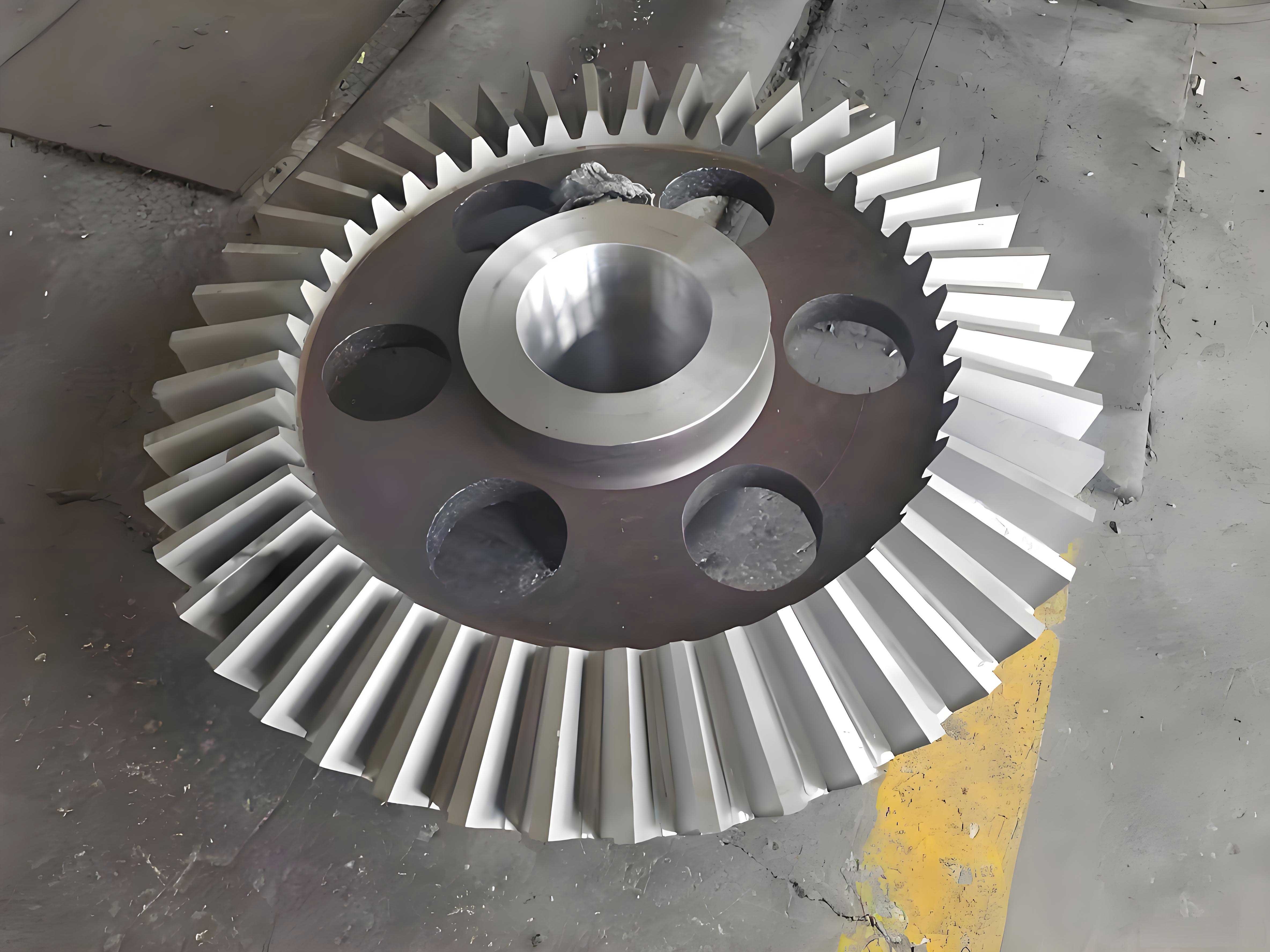
I organize the article around four central tasks. First, I establish a torsional dynamic model of the star herringbone gear system and eliminate rigid-body displacement. Second, I solve the dimensionless differential equations and examine dynamic load, load sharing, bifurcation, phase portraits, Poincare sections, and joint probability density. Third, I apply cell mapping and region discretization to obtain parameter solution domains and state-space basins of attraction. Fourth, I introduce random excitation into the model and evaluate global dynamic behavior when damping, power, input speed, and backlash fluctuate. Throughout the discussion I repeatedly connect the results to miter gears, because miter gears are often used in compact power transmission layouts where backlash, mesh stiffness variation, and load fluctuation can produce complex global responses.
Nomenclature and Core Variables
| Symbol | Meaning | Role in the model |
|---|---|---|
| $$\theta_s$$ | Sun gear rotational displacement | Input rotational coordinate |
| $$\theta_{pi}$$ | Rotational displacement of planet gear i | Planet branch coordinate |
| $$\theta_r$$ | Ring gear rotational displacement | Output rotational coordinate |
| $$x_{spi}$$ | Relative displacement along the mesh line between sun and planet i | External mesh coordinate |
| $$x_{rpi}$$ | Relative displacement along the mesh line between ring and planet i | Internal mesh coordinate |
| $$k_{spi},k_{rpi}$$ | Time-varying mesh stiffness | Parametric excitation |
| $$c_{spi},c_{rpi}$$ | Mesh damping | Dissipative excitation |
| $$b$$ | Backlash | Strong nonlinearity |
| $$e(t)$$ | Comprehensive transmission error | Internal displacement excitation |
| $$\omega_n$$ | Reference time scale | Dimensionless normalization |
| $$L$$ | Reference displacement scale | Dimensionless normalization |
| $$K_v$$ | Dynamic load coefficient | Dynamic load measure |
| $$K_{ls}$$ | Load sharing coefficient | Load distribution measure |
| $$\mathcal{B}$$ | Basin of attraction | Global state-space domain |
| $$C$$ | Cell mapping operator | Global evolution operator |
I adopt the lumped-mass method because it captures the dominant torsional behavior of star herringbone trains while remaining computationally suitable for repeated global mapping. I treat each herringbone gear as two equivalent helical gear halves with opposite helix directions. The left and right halves share a central web, so the axial forces cancel. This modeling choice is also relevant to miter gears when their support stiffness is high and their dominant vibration mode is close to a torsional or rotational mode. In such cases, a torsional representation can provide a useful first approximation before a full three-dimensional miter gear model is constructed.
Dynamic Model of the Star Herringbone Train
I define the rotational coordinate vector as
$$
\mathbf{q} = \left[ \theta_s,\theta_{p1},\theta_{p2},\theta_{p3},\theta_r \right]^T .
$$
The relative displacement along the mesh line for the sun-planet and ring-planet pairs is written as
$$
x_{spi}^{(1)} = \left( r_s\theta_s + r_{pi}\theta_{pi} \right)\cos\beta_1 – e_{spi}^{(1)}(t),
$$
$$
x_{spi}^{(2)} = \left( r_s\theta_s + r_{pi}\theta_{pi} \right)\cos\beta_2 – e_{spi}^{(2)}(t),
$$
$$
x_{rpi}^{(1)} = \left( r_r\theta_r – r_{pi}\theta_{pi} \right)\cos\beta_1 – e_{rpi}^{(1)}(t),
$$
$$
x_{rpi}^{(2)} = \left( r_r\theta_r – r_{pi}\theta_{pi} \right)\cos\beta_2 – e_{rpi}^{(2)}(t),
$$
where the superscripts 1 and 2 denote the two helical halves. The helix angles satisfy
$$
\beta_2 = -\beta_1 .
$$
Using Newton’s second law for each rotational degree of freedom, I obtain the torsional vibration differential equations. For the sun gear,
$$
I_s\ddot{\theta}_s + \sum_{i=1}^{3}\left( k_{spi}x_{spi} + c_{spi}\dot{x}_{spi} \right) r_s \cos\beta = T_s .
$$
For each planet gear,
$$
I_{pi}\ddot{\theta}_{pi} + \left( k_{rpi}x_{rpi} + c_{rpi}\dot{x}_{rpi} \right) r_{pi}\cos\beta – \left( k_{spi}x_{spi} + c_{spi}\dot{x}_{spi} \right) r_{pi}\cos\beta = 0 .
$$
For the ring gear,
$$
I_r\ddot{\theta}_r + \sum_{i=1}^{3}\left( k_{rpi}x_{rpi} + c_{rpi}\dot{x}_{rpi} \right) r_r \cos\beta = -T_r .
$$
I then eliminate the rigid-body displacement by using relative coordinates. This step is important for star herringbone systems because the overall rotation of the train does not contribute to tooth contact deformation. The same elimination procedure is useful for miter gears when a pure torsional model is required for a geared system with intersecting axes.
I introduce the reference time and displacement scales
$$
\omega_n = \sqrt{k_m\left( \frac{1}{M_s} + \frac{1}{M_p} \right)}, \qquad L = 1.0\times 10^{-4}\ \text{m}.
$$
The dimensionless time and displacement are
$$
\tau = \omega_n t, \qquad u = \frac{x}{L}.
$$
The derivatives transform as
$$
\dot{x} = L\omega_n \dot{u}, \qquad \ddot{x} = L\omega_n^2 \ddot{u}.
$$
After eliminating rigid-body motion and normalizing, I write the system in matrix form:
$$
\mathbf{M}\ddot{\mathbf{U}} + \mathbf{C}\dot{\mathbf{U}} + \mathbf{K}\mathbf{g}(\mathbf{U}) = \mathbf{F}.
$$
Here the mass matrix is the identity matrix in dimensionless form, the damping matrix and stiffness matrix are fully populated and symmetric, and the external load vector contains the input and output torque terms. The backlash function is
$$
g(u) =
\begin{cases}
u – \dfrac{b}{2}, & u > \dfrac{b}{2}, \\[6pt]
0, & |u| \le \dfrac{b}{2}, \\[6pt]
u + \dfrac{b}{2}, & u < -\dfrac{b}{2}.
\end{cases}
$$
The time-varying mesh stiffness is represented by a Fourier series:
$$
k(\tau) = k_m\left[ 1 + \varepsilon \sum_{j=1}^{n} a_j \sin\left( j\omega\tau + \phi_0 \right) \right].
$$
The comprehensive transmission error is
$$
e(t) = E\sin\left( \omega t + \phi \right).
$$
The initial mesh phase for the sun-planet and ring-planet pairs is expressed as
$$
\phi_{spi} = \alpha_t + 2\pi(i-1)/N_p,
$$
$$
\phi_{rpi} = -\alpha_t + 2\pi(i-1)/N_p,
$$
where \(N_p\) is the number of planet gears. These phase relations determine how the branches combine in the star train and how the global response evolves under miter gear-like compact layouts.
Numerical Parameters and Dynamic Measures
I select a star herringbone gear system that satisfies the assembly conditions. The main geometric and dynamic parameters are listed below.
| Parameter | Sun gear | Planet gear | Ring gear |
|---|---|---|---|
| Number of components | 1 | 3 | 1 |
| Module | 4 mm | 4 mm | 4 mm |
| Number of teeth | 36 | 32 | 100 |
| Mass | 5.3018 kg | 4.5099 kg | 16.0843 kg |
| Rotational inertia | 0.0226 kg m^2 | 0.0149 kg m^2 | 0.6564 kg m^2 |
| Normal pressure angle | 20 deg | 20 deg | 20 deg |
| Base helix angle | 22.5 deg | 22.5 deg | 22.5 deg |
The mean mesh stiffness is
$$
k_m = 2.0\times 10^9\ \text{N/m}.
$$
The reference mesh damping ratio is
$$
\zeta_m = 0.1.
$$
The physical backlash is
$$
b_0 = 1.0\times 10^{-4}\ \text{m}.
$$
I compute the dynamic load coefficient as
$$
K_v = \frac{F_k + F_c}{F_{in}},
$$
where the elastic mesh force is
$$
F_k = k(\tau)u(\tau)L,
$$
the damping force is
$$
F_c = c\omega_n \dot{u}(\tau)L,
$$
and the static load is
$$
F_{in} = \frac{T}{r}.
$$
I also compute the load sharing coefficient as
$$
K_{ls} = \frac{1}{N}\sum_{i=1}^{N} K_{v,i}.
$$
When I compare star herringbone behavior with miter gears, I note that miter gears usually have intersecting axes and equal speed ratios. Their load-sharing behavior is different, but their sensitivity to backlash and mesh stiffness variation is often similarly significant. Therefore, the dynamic load and load sharing measures introduced here provide a useful template for miter gears in compact transmissions.
Dynamic Response and Bifurcation Analysis
I solve the dimensionless differential equations using the fourth-order Runge-Kutta method. I use phase portraits, Poincare sections, bifurcation diagrams, and joint probability density to identify periodic, multi-periodic, quasi-periodic, and chaotic states. I begin with input speed because the star herringbone system responds strongly to speed changes. The input speed range is
$$
n_1 \in [4000, 20000]\ \text{r/min}.
$$
I summarize the observed bifurcation behavior in the following table.
| Parameter | Range or value | Observed behavior | Dynamic implication |
|---|---|---|---|
| Input speed | 4000 to 7560 r/min | Period-1, period-2, period-4, then chaos through several channels | The system is highly speed-sensitive |
| Input speed | 7560 to 12000 r/min | Short chaos, period-2, jumps, and re-entry into chaos | Jump phenomena occur near narrow speed intervals |
| Input speed | 12000 to 20000 r/min | Period-2, period-4, chaos, then inverse bifurcation to period-2 and period-1 | Higher speed can stabilize the response after complex transitions |
| Input power | 1500 to 4000 kW | Chaos, quasi-period, period-doubling, and inverse bifurcation | Increasing power promotes stable periodic motion |
| Mesh damping ratio | 0.05 to 0.20 | Chaos, quasi-period, period-2, and period-1 | Larger damping suppresses chaotic vibration |
| Stiffness fluctuation | 0.1 to 0.3 and above | Period-4 followed by chaos | Small stiffness fluctuation is preferable |
| Backlash | 0.8 to 1.5 dimensionless | Quasi-period-2 with jumps | Backlash increases vibration amplitude |
For the speed sweep, I observe period-doubling, inverse bifurcation, jumps, and chaos. The system enters chaos from multiple period-doubling channels, and the Poincare section exhibits fractal point sets. The phase trajectory does not overlap completely in the chaotic state, which indicates repeated local winding and sensitive dependence on initial conditions. These features are also common in miter gears when backlash and mesh stiffness variation are present, although the axis geometry of miter gears can introduce additional three-dimensional effects.
I write the Poincare map as
$$
\mathbf{P}: \Sigma \rightarrow \Sigma, \qquad \mathbf{x}_{n+1} = \mathbf{P}(\mathbf{x}_n).
$$
A period-K attractor satisfies
$$
\mathbf{x}_{n+K} = \mathbf{x}_n.
$$
In numerical computation I use the tolerance condition
$$
\left\| \mathbf{x}_{n+K} – \mathbf{x}_n \right\| < \epsilon.
$$
I also estimate the joint probability density from the Poincare section after 300 steady-state periods. For a period-4 attractor, the joint probability density has four nearly equal vertical peaks. For a chaotic attractor, the density forms irregular peak groups or a broad cluster. This provides a qualitative verification of the attractor type and helps distinguish coexisting attractors from a single complex attractor. In miter gears, similar probability density structures can be used to identify whether measured vibration is periodic, quasi-periodic, or chaotic.
Effect of Input Power and Mesh Damping
I increase the input power from 1500 kW to 4000 kW. The system passes through chaos, quasi-periodic motion, period-doubling, and finally inverse bifurcation into stable periodic motion. As power increases, the vibration amplitude fluctuations decrease, and the dynamic response becomes more regular. This suggests that a sufficiently high input power can improve the steady-state stability of the star herringbone train. The same trend may appear in miter gears when the transmitted torque is high enough to keep the teeth in contact and reduce the influence of backlash.
For mesh damping, I vary the damping ratio from 0.05 to 0.20. At low damping the system is chaotic. As damping increases, the system exits chaos through inverse bifurcation, then becomes quasi-periodic, period-2, and finally period-1. This result indicates that a larger mesh damping ratio is beneficial for suppressing chaotic vibration and reducing amplitude. In miter gears, increased damping from lubricant films or material damping can similarly reduce nonlinear impacts, although excessive damping may increase power loss.
Effect of Stiffness Fluctuation and Backlash
I define the stiffness fluctuation coefficient as \(\varepsilon\). When \(\varepsilon\) lies between 0.1 and 0.3, the system remains in period-4 motion. When \(\varepsilon\) exceeds 0.3, the response enters chaos and the vibration amplitude grows. Therefore, I recommend selecting a relatively small stiffness fluctuation coefficient during design. For miter gears, tooth contact stiffness variation caused by manufacturing errors and load distribution can produce similar parametric excitation. Reducing stiffness fluctuation is therefore a general design objective for both star herringbone systems and miter gears.
For backlash, I vary the dimensionless backlash from 0.8 to 1.5. The system remains quasi-period-2, but jump phenomena occur, and the vibration amplitude increases with backlash. A smaller backlash helps reduce impact and noise. However, if backlash is too small, the risk of interference and lubrication failure increases. Therefore, an optimal backlash range should be selected by considering both dynamic stability and practical lubrication. This trade-off is especially important for miter gears, which often operate in compact housings where thermal expansion and misalignment can change the effective backlash.
Experimental Verification
I verify the dynamic model by building a star herringbone gear transmission test rig. I use an AC variable-frequency motor, a magnetic powder brake, a gearbox, accelerometers, a data acquisition unit, and a computer. I place accelerometers near the bearing end covers along the direction parallel to the mesh line. I measure the relative vibration acceleration of the sun-planet mesh pair by subtracting the planet acceleration from the sun acceleration. I test three input speeds: 1000 r/min, 1250 r/min, and 1500 r/min. The corresponding mesh frequencies are listed below.
| Input speed | First mesh frequency | Second mesh frequency | Sampling frequency |
|---|---|---|---|
| 1000 r/min | 2352 Hz | 4704 Hz | 6000 Hz |
| 1250 r/min | 2940 Hz | 5880 Hz | 7500 Hz |
| 1500 r/min | 3528 Hz | 7056 Hz | 9000 Hz |
I apply a load of 2 N m and record the acceleration signals. After fast Fourier transform, I compare the measured frequency-domain amplitudes with the theoretical results. The amplitudes agree well, with small deviations caused by manufacturing errors, assembly errors, bearings, couplings, and neglected friction. The agreement confirms that the dynamic model is reliable and that the subsequent global analysis is meaningful. Although the experiment is performed on a star herringbone system, the verification philosophy also applies to miter gears, where similar acceleration measurements can be used to validate global dynamic models.
Cell Mapping and Region Discretization
To reveal the global dynamic characteristics, I use cell mapping and region discretization. A non-autonomous nonlinear system can be written as
$$
\dot{\mathbf{X}}(t) = \mathbf{f}\left( \mathbf{X}(t), t, \boldsymbol{\alpha} \right),
$$
where \(\mathbf{X}\) is the state vector and \(\boldsymbol{\alpha}\) is the parameter vector. I discretize the parameter space or state space into small cells. Each cell is mapped forward under the Poincare map. A simple cell mapping operator \(C\) is defined by
$$
Z_{k+1} = C(Z_k).
$$
A periodic cell of period \(K\) satisfies
$$
Z_{k+K} = Z_k.
$$
I identify the attractor type by checking the distance between successive Poincare points. If the distance between four consecutive points is smaller than a tolerance, I classify the cell as a periodic attractor. If no periodicity is found within the maximum number of mappings, I classify the cell as chaotic. If a cell differs from its neighbors in attractor type, I mark it as a boundary cell. This boundary detection is important because the basin boundaries in star herringbone systems can be fractal, and the same is often true for miter gears with clearance and time-varying stiffness.
I summarize the cell classification labels in the following table.
| Label | Attractor type | Meaning |
|---|---|---|
| P1 | Period-1 | Steady periodic motion with one Poincare point |
| P2 | Period-2 | Steady periodic motion with two Poincare points |
| P4 | Period-4 | Steady periodic motion with four Poincare points |
| Pn | Multi-periodic | Period greater than four |
| Chaotic | Chaotic | No finite periodicity detected |
Parameter Solution Domains
I construct two-dimensional parameter solution domains for speed-power, speed-damping, and power-damping combinations. I discretize each parameter plane into \(200 \times 200\) regular cells. For each parameter cell I set the initial state to zero and map the system to its steady state. The resulting domains show which parameter combinations lead to period-1, period-2, period-4, multi-periodic, or chaotic motion.
The speed-power solution domain shows that the system is highly sensitive to input speed. Along the speed axis, the response changes frequently among period-1, period-2, period-4, and chaos. Along the power axis, increasing power generally drives the system toward period-1 or period-2 motion. At high speed, however, the response becomes sensitive to power again, and period-1, period-4, and period-5 domains alternate. Therefore, high-speed operation requires careful selection of input power. In miter gears, a similar two-parameter map can be used to select speed and load combinations that avoid chaotic miter gear vibration.
The speed-damping solution domain shows that increasing damping generally reduces chaotic regions and promotes period-1 and period-2 motion. However, at high speed, period-3 and period-4 domains can be nested inside period-2 domains, and small damping changes can cause frequent transitions. This indicates that damping is helpful but must be chosen with attention to speed-dependent bifurcation. For miter gears, damping optimization should therefore be performed together with speed selection rather than independently.
The power-damping solution domain shows a clear trend: when power and damping are both small, chaos dominates. As power and damping increase, the chaos region shrinks and period-2 and period-4 domains expand. When damping is greater than about 0.17, the system tends to remain period-2 regardless of power within the studied range. This result suggests that a properly selected damping ratio can make the global behavior robust against power fluctuation. The same principle can guide miter gear design when miter gears are used in variable-load systems.
I summarize selected parameter-domain observations in the table below.
| Parameter plane | Main domains | Coupling effect | Design guidance |
|---|---|---|---|
| Speed and power | P1, P2, P4, Pn, chaotic | Speed strongly controls transitions; power stabilizes at moderate speed | Avoid high-speed chaotic bands; select adequate power |
| Speed and damping | P1, P2, P4, Pn, chaotic | Damping weakens chaos but high-speed nesting remains | Increase damping while avoiding high-speed boundary regions |
| Power and damping | P2, P4, Pn, chaotic | Both parameters suppress chaos when increased | Choose moderate power and sufficiently high damping |
I observe that some solution domains are nested. For example, a period-4 domain may appear inside a period-2 domain. This means that global optimization cannot rely only on average trends. Local attractor jumps must also be considered. The same caution applies to miter gears, where a small parameter change can move the system from a safe periodic basin into a chaotic or high-amplitude basin.
State-Space Basins of Attraction
I study the state-space basins of attraction for the star herringbone system. I discretize the state space into \(200 \times 200\) cells over
$$
x \in [-1,1], \qquad \dot{x} \in [-1,1].
$$
For each state cell, I solve the system and determine the final attractor. The basin of attraction of an attractor \(A\) is
$$
\mathcal{B}(A) = \left\{ (x,\dot{x}) \mid \lim_{n\to\infty} \mathbf{P}^n(x,\dot{x}) \in A \right\}.
$$
At a speed of 9000 r/min and a power of 2800 kW, the global basin contains period-2, multi-periodic, and chaotic domains. The chaotic basin occupies about 60 percent of the state space, while the period-2 basin occupies about 21 percent. The basins are interwoven, which means that the system is highly sensitive to initial conditions. When power increases to 3000 kW, the chaotic basin shrinks to about 7 percent, and multi-periodic motion becomes dominant. When power increases to 3200 kW, the period-2 and period-4 basins expand to about 64 percent of the state space, and the chaotic basin disappears. This indicates that increasing power can suppress chaos and reduce initial-condition sensitivity.
I summarize the basin evolution under power in the following table.
| Power | Period-2 basin | Period-4 basin | Chaotic basin | Main global feature |
|---|---|---|---|---|
| 2800 kW | 21 percent | 1 percent | 60 percent | Chaos-dominated, strongly interwoven basins |
| 3000 kW | 23 percent | Small | 7 percent | Multi-periodic domains expand, chaos weakens |
| 3200 kW | 34 percent | 30 percent | 0 percent | Periodic domains dominate, initial sensitivity decreases |
For damping, I study the basin evolution at a fixed power of 3000 kW. At a damping ratio of 0.08, the chaotic basin occupies about 85 percent of the state space. At a damping ratio of 0.10, the chaotic basin is greatly reduced. At a damping ratio of 0.12, the global domain is composed entirely of period-2 and period-4 basins. The period-2 basin occupies about 35 percent, and the period-4 basin occupies about 65 percent. The basin boundaries become simpler, and the system becomes less sensitive to initial conditions. This shows that increasing damping can effectively suppress chaos and stabilize the global response. For miter gears, increasing damping through lubrication and material selection may similarly simplify the basin structure and reduce the risk of chaotic miter gear vibration.
I summarize the damping basin evolution in the following table.
| Damping ratio | Chaotic basin | Period-2 basin | Period-4 basin | Global feature |
|---|---|---|---|---|
| 0.08 | 85 percent | Small | Small | Chaos dominates |
| 0.10 | 7 percent | 23 percent | Small | Chaos reduces, multi-periodic domains expand |
| 0.12 | 0 percent | 35 percent | 65 percent | All periodic, simple basin structure |
I find that the global basin evolution is consistent with the local bifurcation path. When a local bifurcation indicates a transition from chaos to period-2 motion, the corresponding basin of period-2 expands. When a local bifurcation indicates a transition from period-2 to period-4 motion, the period-4 basin grows. This consistency confirms that cell mapping is a reliable tool for global analysis. It also suggests that miter gear designers can use local bifurcation diagrams to guide global basin optimization, provided that the parameter domain is not too large and the dominant nonlinearities are included.
Random Excitation and Global Dynamics
In real gear systems, excitation parameters are not perfectly constant. Manufacturing errors, transmission errors, vibration coupling, and operating condition changes cause random fluctuations. I introduce random excitation into the star herringbone model to represent this reality. I use the central limit theorem and the limit approximation method to generate pseudo-random numbers that approximately follow a normal distribution. For independent uniform random variables \(U_i\) on \([0,1]\), the standardized sum is
$$
\xi = \sqrt{\frac{12}{n}}\left( \sum_{i=1}^{n} U_i – \frac{n}{2} \right).
$$
For \(n=12\), this reduces to
$$
\xi = \sum_{i=1}^{12} U_i – 6 \sim N(0,1).
$$
A normal random excitation with mean \(\mu\) and standard deviation \(\sigma\) is then
$$
\eta = \mu + \sigma \xi.
$$
I generate one random number per mesh cycle and check whether it lies within the prescribed lower and upper limits. If it does, I assign it to the excitation parameter. If it does not, I regenerate the number until the boundary condition is satisfied. I then solve the random nonlinear system and apply cell mapping to obtain the global basin. In this way I can compare deterministic and random global dynamics.
Random Damping
I first let the mesh damping ratio follow
$$
K_{em} \sim N(0.1, 0.0002^2).
$$
The fluctuation limits are 0.0994 and 0.1006. The global basin still contains period-2, period-4, and multi-periodic domains, but the boundaries become more irregular. The period-2 basin occupies about 33 percent, and the period-4 and period-6 basins together occupy about 31 percent. Multi-periodic domains occupy about 36 percent. Compared with the deterministic case, the basin structure is slightly degraded. The attractor begins to fluctuate, and the response tends toward quasi-period-2 motion.
When the variance increases to \(0.0004^2\), the global basin changes more significantly. Period-4, multi-periodic, and chaotic domains appear. The period-4 basin occupies about 32 percent, multi-periodic about 40 percent, and chaotic about 1.7 percent. The period-2 basin decreases to about 25 percent. The attractor fluctuates more strongly and approaches quasi-period-2 or even chaotic behavior. This shows that random damping fluctuation can worsen the global dynamic characteristics, and the degree of worsening increases with variance. For miter gears, random damping changes caused by lubrication variation or temperature variation can produce a similar effect, so miter gear lubrication should be controlled carefully.
Random Power
I let the input power follow
$$
P \sim N(3200, 3^2)\ \text{kW}.
$$
The fluctuation limits are 3190 kW and 3210 kW. The period-2 basin increases slightly to about 34.5 percent, and the period-4 basin increases to about 31 percent. A small number of period-6 cells appear, about 0.3 percent. Some period-4 and multi-periodic cells switch to period-2, while some period-2 cells switch to period-4. The basin boundaries become more numerous, but the overall global behavior does not deteriorate. The attractor remains period-2. This indicates that small random fluctuations in input power are acceptable. In miter gear systems, load fluctuations of a few percent may not seriously damage the global dynamic stability if the mean operating point is well chosen.
Random Input Speed
I let the input speed follow
$$
n_1 \sim N(9000, 3^2)\ \text{r/min}.
$$
At 9000 r/min, the deterministic system lies near the boundary between periodic and chaotic domains. Therefore, even a small random speed fluctuation causes severe global deterioration. The global basin becomes dominated by chaotic and multi-periodic domains. The chaotic basin occupies about 63 percent, and the multi-periodic basin occupies about 20 percent. The period-2 and period-4 basins almost disappear. The basin structure becomes tangled and irregular, and the attractor becomes chaotic. This result shows that the star herringbone system is extremely sensitive to input speed. For miter gears, speed fluctuation can similarly move a well-designed miter gear pair into a chaotic region, especially when the nominal speed is near a bifurcation boundary.
Random Backlash
I let the dimensionless backlash follow
$$
b \sim N(1, 0.002^2).
$$
Backlash is a strong nonlinear factor. Even a very small random fluctuation causes significant deterioration. The global basin becomes dominated by chaotic attractors, occupying about 69 percent. Multi-periodic attractors occupy about 18 percent, and periodic attractors occupy only about 13 percent. The basin structure is scattered, and no complete periodic basin remains. The attractor becomes chaotic. This shows that backlash random fluctuation is highly detrimental. To avoid chaotic miter gear or star herringbone vibration, backlash should be controlled within a small range, and random variation should be minimized through high-precision manufacturing and proper thermal compensation.
I summarize the random excitation results in the following table.
| Random parameter | Distribution | Global effect | Attractor change | Practical guidance |
|---|---|---|---|---|
| Damping ratio | $$N(0.1,0.0002^2)$$ | Slight basin irregularity | Period-2 tends to quasi-period-2 | Control lubrication and damping variation |
| Damping ratio | $$N(0.1,0.0004^2)$$ | Chaotic cells appear, multi-periodic domains expand | Quasi-period-2 with chaos risk | Reduce damping fluctuation |
| Input power | $$N(3200,3^2)$$ | Minor basin rearrangement, no severe degradation | Period-2 remains | Small power fluctuation is acceptable |
| Input speed | $$N(9000,3^2)$$ | Chaotic basin dominates | Chaotic attractor | Avoid boundary speeds, improve speed precision |
| Backlash | $$N(1,0.002^2)$$ | Chaotic basin dominates, basins scattered | Chaotic attractor | Minimize backlash fluctuation |
Global Design Implications for Miter Gears and Star Herringbone Systems
The global analysis shows that star herringbone and miter gears share several design principles. First, avoid parameter regions near basin boundaries. Near a boundary, a small change in speed, backlash, or damping can cause a jump from a periodic attractor to a chaotic attractor. Second, increase damping when possible, because damping generally shrinks chaotic basins and simplifies basin boundaries. Third, control backlash tightly, because backlash is a strong nonlinearity and its random fluctuation is especially harmful. Fourth, use enough power or torque to keep teeth in contact and stabilize the periodic response. Fifth, use parameter-domain maps to select operating points rather than relying only on one-dimensional bifurcation diagrams. These principles are valid for miter gears used in compact, high-speed, and high-load systems, even though the detailed geometry of miter gears differs from that of star herringbone gears.
I also note that the global basin structure can be used as a design objective. Instead of only minimizing vibration amplitude at a single operating point, I can maximize the area of the safe periodic basin. A large periodic basin means that the system is robust to initial-condition changes and small parameter fluctuations. This is particularly important for miter gears, which often operate under varying load and speed conditions. A miter gear pair with a large safe basin is less likely to jump into a chaotic or high-amplitude state when the operating conditions change.
Mathematical Summary of the Global Method
For clarity, I summarize the global method in a compact mathematical form. The deterministic system is
$$
\mathbf{M}\ddot{\mathbf{U}} + \mathbf{C}\dot{\mathbf{U}} + \mathbf{K}\mathbf{g}(\mathbf{U}) = \mathbf{F}(\tau).
$$
The dimensionless state vector is
$$
\mathbf{y} = \left[ \mathbf{U}^T, \dot{\mathbf{U}}^T \right]^T.
$$
The first-order form is
$$
\dot{\mathbf{y}} = \mathbf{f}(\mathbf{y},\tau,\boldsymbol{\alpha}).
$$
The Poincare map is
$$
\mathbf{y}_{n+1} = \mathbf{P}(\mathbf{y}_n,\boldsymbol{\alpha}).
$$
The parameter-domain solution is
$$
\mathcal{D}(\boldsymbol{\alpha}) = \left\{ \boldsymbol{\alpha} \mid \mathbf{P}^n(\mathbf{y}_0,\boldsymbol{\alpha}) \in A_j \right\}.
$$
The state-space basin is
$$
\mathcal{B}(A_j) = \left\{ \mathbf{y}_0 \mid \lim_{n\to\infty} \mathbf{P}^n(\mathbf{y}_0,\boldsymbol{\alpha}) \in A_j \right\}.
$$
For random excitation, the parameter is
$$
\boldsymbol{\alpha} = \boldsymbol{\alpha}_0 + \boldsymbol{\sigma}\boldsymbol{\xi},
$$
where \(\boldsymbol{\xi}\) is a standard normal random vector. The random global domain is then obtained by cell mapping over many realizations. This formulation is general and can be applied to miter gears by replacing the torsional coordinates with the appropriate miter gear coordinates and by including the intersecting-axis mesh geometry.
Key Findings
I find that the star herringbone gear transmission system exhibits rich nonlinear dynamic behavior, including period-doubling, inverse bifurcation, jumps, quasi-periodicity, and chaos. Input speed is the most sensitive parameter. Increasing input power and mesh damping generally stabilizes the system. Increasing stiffness fluctuation and backlash generally destabilizes the system. The dynamic load and load sharing coefficients confirm that the sun-planet mesh and ring-planet mesh respond differently, and that the sun-planet mesh can be more strongly affected by impact. Experimental acceleration measurements agree with theoretical results, which validates the model.
For global behavior, the parameter solution domains and state-space basins reveal that the system can transition between periodic and chaotic states through narrow boundary regions. Basin boundaries are often irregular and may be fractal. Increasing power and damping expands periodic basins and shrinks chaotic basins. Increasing speed or backlash can produce the opposite effect. Some basins are nested, so local attractor jumps must be considered during optimization. The global method provides a more comprehensive view than one-dimensional bifurcation analysis alone.
For random excitation, damping and power fluctuations cause only mild degradation, while input speed and backlash fluctuations cause severe degradation. When input speed is near a basin boundary, a small random fluctuation can push the system into chaos. When backlash fluctuates, the chaotic basin can dominate the entire state space. Therefore, speed precision and backlash control are critical. Input power fluctuation is relatively benign, and small variations can even improve the basin structure in some cases. These conclusions are relevant to miter gears because miter gears also rely on precise speed control, controlled backlash, and adequate damping for stable operation.
Conclusion
I have presented a global dynamic study of a star herringbone gear transmission system under multi-source excitation and extended the interpretation to miter gears. I built a torsional dynamic model, eliminated rigid-body displacement, normalized the equations, and solved them with a fourth-order Runge-Kutta method. I analyzed dynamic load, load sharing, bifurcation, phase portraits, Poincare sections, and joint probability density. I then applied cell mapping and region discretization to obtain parameter solution domains and state-space basins of attraction. Finally, I introduced random excitation and evaluated the global effects of random damping, random power, random input speed, and random backlash. The results show that global analysis can reveal attractor transitions and basin evolution that are not visible in local analysis alone. For both star herringbone systems and miter gears, the safest design strategy is to select operating points away from basin boundaries, increase damping, control backlash, and use parameter-domain maps to guide speed and load selection.