
In this work, I study the dynamic behavior of a motor-driven helical rack and pinion feed system used in large CNC machines. The central problem I address is how the electromechanical coupling between an AC synchronous servo motor and a helical rack and pinion transmission affects the dynamic transmission error of the feed axis. I build a lumped-parameter mechanical model, a vector-controlled motor model, and a coupled electromechanical simulation. I also perform experiments on a CNC machine axis. The results show that the meshing error of the rack and pinion gears is the main source of dynamic error, while the shaft frequency and mesh frequency dominate the error spectrum.
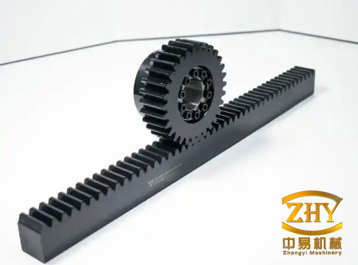
The feed system I consider consists of an AC synchronous servo motor, a reducer, a helical pinion, a fixed rack, and a moving load. The motor supplies torque; the reducer transmits torque to the pinion; the pinion rotates and meshes with the fixed rack; because the rack is fixed, the pinion translates and drives the load. This arrangement is common in long-stroke, heavy-duty machines because rack and pinion gears provide high load capacity and stable motion. A representative rack and pinion configuration is shown below.
I use a first-principles approach. First, I derive the mechanical dynamics of the helical rack and pinion transmission. Second, I compute the time-varying mesh stiffness using the potential energy method and the slicing-integrating method. Third, I include mesh error as an internal excitation. Fourth, I model the AC synchronous servo motor with vector control and a double closed-loop strategy. Fifth, I combine the motor and the rack and pinion mechanics into a single electromechanical system. Finally, I compare simulation and experimental results for several feed speeds.
Mechanical model of the helical rack and pinion feed system. I adopt a lumped-parameter method. The motor shaft, the pinion, and the load are treated as rigid bodies connected by stiffness and damping elements. The governing equations are
$$
\begin{aligned}
J_{mx}\ddot{\theta}_{mx} &= T_{ex} – k_{rx}\left(\theta_{mx}-i_x\theta_{gx}\right) – c_{rx}\left(\dot{\theta}_{mx}-i_x\dot{\theta}_{gx}\right),\\
J_{gx}\ddot{\theta}_{gx} &= i_x\left[k_{rx}\left(\theta_{mx}-i_x\theta_{gx}\right)+c_{rx}\left(\dot{\theta}_{mx}-i_x\dot{\theta}_{gx}\right)\right] – f_{nx}r_{gx},\\
m_{gx}\ddot{x}_{gx} &= f_{nx} – k_{sx}\left(x_{gx}-x_{lx}\right) – c_{sx}\left(\dot{x}_{gx}-\dot{x}_{lx}\right),\\
m_{lx}\ddot{x}_{lx} &= k_{sx}\left(x_{gx}-x_{lx}\right) + c_{sx}\left(\dot{x}_{gx}-\dot{x}_{lx}\right) – f_{lx}.
\end{aligned}
$$
Here, \(T_{ex}\) is the driving torque from the motor, \(k_{rx}\) is the torsional stiffness of the reducer, \(c_{rx}\) is the torsional damping of the reducer, \(i_x\) is the reduction ratio, \(f_{nx}\) is the dynamic mesh force between the helical pinion and the rack, \(r_{gx}\) is the pitch radius of the pinion, \(k_{sx}\) is the support stiffness between the pinion and the load, \(c_{sx}\) is the support damping, \(f_{lx}\) is the resistance force on the load, \(J_{mx}\) is the motor inertia, \(J_{gx}\) is the pinion inertia, \(m_{gx}\) is the pinion mass, and \(m_{lx}\) is the load mass. The dynamic mesh force is written as
$$
f_{nx}=k_{nx}\cos\alpha_n\left(r_{gx}\theta_{gx}-x_{gx}-e_{nx}\cos\alpha_n\right)
+c_{nx}\cos\alpha_n\left(r_{gx}\dot{\theta}_{gx}-\dot{x}_{gx}-\dot{e}_{nx}\cos\alpha_n\right).
$$
In this expression, \(k_{nx}\) is the normal mesh stiffness of the helical rack and pinion, \(c_{nx}\) is the normal mesh damping, \(\alpha_n\) is the normal pressure angle, and \(e_{nx}\) is the mesh error. The helical angle introduces a gradual engagement and disengagement process, so the mesh stiffness and mesh error are both time-varying. This time-varying behavior is essential for accurate prediction of the dynamic error in rack and pinion gears.
Time-varying mesh stiffness by potential energy and slice integration. Because the rack has an infinite involute radius, I replace it with an equivalent helical gear of the same size as the pinion. The total mesh stiffness of the helical rack and pinion is obtained by combining bending stiffness, shear stiffness, axial compression stiffness, Hertz contact stiffness, and fillet foundation stiffness. The corresponding expressions are
$$
k_b=\sum_{i=1}^{N}\frac{1}{\int_{-\alpha_1′}^{\alpha_2}\frac{3\cos\alpha(\alpha_2-\alpha)\left(1+\cos\alpha_1’\left((\alpha_2-\alpha)\sin\alpha-\cos\alpha\right)\right)^2}{2E\Delta z\left(\sin\alpha+(\alpha_2-\alpha)\cos\alpha\right)^3}\,d\alpha},
$$
$$
k_s=\sum_{i=1}^{N}\frac{1}{\int_{-\alpha_1′}^{\alpha_2}\frac{1.2(1+v)(\alpha_2-\alpha)\cos\alpha\cos^2\alpha_1′}{E\Delta z\left(\sin\alpha+(\alpha_2-\alpha)\cos\alpha\right)}\,d\alpha},
$$
$$
k_a=\sum_{i=1}^{N}\frac{1}{\int_{-\alpha_1′}^{\alpha_2}\frac{(\alpha_2-\alpha)\cos\alpha\sin^2\alpha_1′}{2E\Delta z\left(\sin\alpha+(\alpha_2-\alpha)\cos\alpha\right)}\,d\alpha},
$$
$$
k_h=\frac{\pi E L_{ct}}{4(1-\nu^2)}.
$$
Here, \(E\) is Young’s modulus, \(\nu\) is Poisson’s ratio, \(L_{ct}\) is the length of the contact line, \(\Delta z=L_{ct}\cos\beta_b/N\) is the projected length of each slice, \(\beta_b\) is the base helix angle, \(N\) is the number of slices, \(\alpha_1’\) is the angle between the mesh force and the tangential direction, and \(\alpha_2\) is the half base tooth angle. The fillet foundation stiffness is calculated from the classical two-dimensional analytical formula:
$$
k_f=\frac{E\Delta z}{\cos^2\alpha_1′}\frac{1}{L\left(\frac{\mu_f}{s_f}\right)^2+M\left(\frac{\mu_f}{s_f}\right)+P\left(1+Q\tan\alpha_1’\right)}.
$$
The parameters \(\mu_f\), \(s_f\), \(L\), \(M\), \(P\), and \(Q\) depend on the gear geometry and are evaluated from standard formulas. The total mesh stiffness of a single tooth pair is the series combination of \(k_b\), \(k_s\), \(k_a\), \(k_h\), and \(k_f\). The overall time-varying mesh stiffness of the helical rack and pinion is then obtained by summing the contributions of all engaged tooth pairs. The helical gear parameters I use are listed in Table 1.
| Parameter | Symbol | Value | Unit |
|---|---|---|---|
| Normal module | \(m_n\) | 2 | mm |
| Normal pressure angle | \(\alpha_n\) | 20 | deg |
| Helix angle | \(\beta\) | 19.5283 | deg |
| Number of teeth | \(N_1\) | 30 | – |
| Face width | \(B\) | 28 | mm |
| Young’s modulus | \(E\) | \(2.06\times10^{11}\) | Pa |
| Poisson’s ratio | \(\nu\) | 0.25 | – |
| Mass | \(m\) | 0.7 | kg |
For a pinion translation speed of 50 mm/s, I compute the time-varying mesh stiffness of the helical rack and pinion. The single-pair stiffness and the combined stiffness over one mesh period show clear periodic variation. To validate the calculation, I compare the average mesh stiffness with the value from the mechanical design handbook. The comparison is given in Table 2.
| Method | Average mesh stiffness (N/m) | Difference (N/m) | Error rate (%) |
|---|---|---|---|
| ISO standard | \(5.009\times10^{8}\) | — | — |
| Potential energy and slice integration | \(5.0925\times10^{8}\) | \(0.0835\times10^{8}\) | 1.67 |
The error rate is only 1.67 %, so the computed time-varying mesh stiffness is reliable for the dynamic analysis of rack and pinion gears.
Mesh error of the helical rack and pinion. The mesh error is represented as a superposition of sinusoidal components at shaft frequency and mesh frequency:
$$
e(t)=0.5F_p\sin\left(2\pi\omega_a t+\phi_a\right)+0.5f’\sin\left(2\pi\omega_n t+\phi_n\right).
$$
Here, \(F_p\) is the total cumulative pitch deviation, \(f’\) is the single-tooth tangential composite deviation, \(\omega_a\) is the shaft frequency, \(\omega_n\) is the mesh frequency, and \(\phi_a\) and \(\phi_n\) are initial phases. In this study, the initial phases are zero. For a six-grade machining accuracy, I use \(F_p=26\ \mu\text{m}\) and \(f’=10.24\ \mu\text{m}\). These values are consistent with standard design data for rack and pinion gears.
Mechanical simulation. I implement the mechanical equations in Simulink. The time-varying mesh stiffness is supplied as a vector to speed up the solution. I set a constant motor torque of \(0.64\ \text{N}\cdot\text{m}\) and balance the load force with the driving force. The solver is ode45. The load displacement error is periodic with a micro-level amplitude. The frequency spectrum of the load displacement shows that the shaft frequency \(f_a=0.25\ \text{Hz}\) and the mesh frequency \(f_n=7.5\ \text{Hz}\) are the main low-frequency components. This agrees with the internal excitation frequencies of the rack and pinion gears. The mechanical parameters used in the simulation are listed in Table 3.
| Parameter | Symbol | Value | Unit |
|---|---|---|---|
| Motor inertia | \(J_{mx}\) | \(1.7\times10^{-5}\) | kg·m\(^2\) |
| Pinion inertia | \(J_{gx}\) | \(3.7703\times10^{-4}\) | kg·m\(^2\) |
| Pinion mass | \(m_{gx}\) | 0.7 | kg |
| Load mass | \(m_{lx}\) | 300 | kg |
| Reducer torsional stiffness | \(k_{rx}\) | 24064 | N·m/rad |
| Support stiffness | \(k_{sx}\) | \(4.843\times10^{9}\) | N/m |
| Reducer torsional damping | \(c_{rx}\) | 0.041 | N·m·s/rad |
| Support damping | \(c_{sx}\) | 3489.7 | N·s/m |
| Reduction ratio | \(i_x\) | 50 | – |
The mechanical simulation confirms that the internal excitations of the rack and pinion gears directly influence the output motion. In particular, the mesh error changes the amplitude of the displacement fluctuation, while the time-varying mesh stiffness changes the frequency content. These effects are important for precision feed drives.
AC synchronous servo motor model. I model the motor using vector control. The three-phase stator currents are transformed from the natural A-B-C frame to the stationary \(\alpha\)-\(\beta\) frame by the Clark transformation:
$$
T_{\text{Clark}}=\frac{2}{3}
\begin{bmatrix}
1 & -\frac{1}{2} & -\frac{1}{2}\\
0 & \frac{\sqrt{3}}{2} & -\frac{\sqrt{3}}{2}\\
\frac{\sqrt{2}}{2} & \frac{\sqrt{2}}{2} & \frac{\sqrt{2}}{2}
\end{bmatrix}.
$$
Then the stationary frame is rotated to the synchronous \(d\)-\(q\) frame by the Park transformation:
$$
T_{\text{Park}}=
\begin{bmatrix}
\cos\theta_e & \sin\theta_e\\
-\sin\theta_e & \cos\theta_e
\end{bmatrix}.
$$
Here, \(\theta_e\) is the electrical rotor angle. The inverse transformations recover the three-phase commands. The electromagnetic torque is
$$
T_e=\frac{3}{2}p_n i_q\left[i_d\left(L_d-L_q\right)+\psi_f\right],
$$
where \(p_n\) is the number of pole pairs, \(i_d\) and \(i_q\) are the \(d\)- and \(q\)-axis currents, \(L_d\) and \(L_q\) are the corresponding inductances, and \(\psi_f\) is the permanent-magnet flux linkage. The mechanical equation of the motor shaft is
$$
J\frac{d\omega_m}{dt}=T_e-T_L,
$$
where \(J\) is the motor inertia, \(\omega_m\) is the mechanical angular speed, and \(T_L\) is the load torque. The motor parameters are given in Table 4.
| Parameter | Symbol | Value | Unit |
|---|---|---|---|
| \(d\)-axis inductance | \(L_d\) | 0.02682 | H |
| \(q\)-axis inductance | \(L_q\) | 0.02682 | H |
| Stator resistance | \(R\) | 18.7 | Ω |
| Motor inertia | \(J\) | \(1.7\times10^{-5}\) | kg·m\(^2\) |
| Pole pairs | \(p_n\) | 2 | – |
| Flux linkage | \(\psi_f\) | 0.1717 | V·s/rad |
| Speed proportional gain | \(P_\omega\) | 0.013 | – |
| \(q\)-axis current proportional gain | \(P_{iq}\) | 200 | – |
| \(d\)-axis current proportional gain | \(P_{id}\) | 200 | – |
| Speed integral gain | \(I_\omega\) | 1.3 | – |
| \(d\)-axis current integral gain | \(I_{id}\) | 10000 | – |
| \(q\)-axis current integral gain | \(I_{iq}\) | 10000 | – |
I simulate the motor with an initial speed of 500 r/min and an initial load of \(0.2\ \text{N}\cdot\text{m}\). After 0.4 s, the speed command changes to 750.73 r/min. After 0.6 s, the load torque changes to \(0.64\ \text{N}\cdot\text{m}\). The motor reaches the commanded speed and torque within about 0.05 s after each change. The step response shows a maximum overshoot of 2.6 %, a peak time of 1.3 ms, and a rise time and settling time of about 20 ms. These results indicate that the vector-controlled motor has fast response, small overshoot, and good steady-state accuracy. The frequency spectrum of the motor speed at 750.73 r/min contains a fundamental component at 150 Hz and several harmonics.
Electromechanical coupling. I connect the motor model and the helical rack and pinion model in series. The motor speed is the input to the mechanical system, and the load torque is fed back to the motor. This forms a closed-loop electromechanical system. The coupling equations can be summarized as
$$
\begin{aligned}
\omega_e &= \omega_m,\\
T_{\text{load}} &= T_L,\\
v_{\text{load}} &= \dot{x}_{lx},\\
T_{ex} &= T_e.
\end{aligned}
$$
I set the motor speed to 750.73 r/min and include a friction resistance of 313.6 N. The ideal load speed is 50 mm/s, so after 10 s the load should move 500 mm. The simulated load displacement matches this value. I compare the commanded displacement \(v=0.05t\) with the simulated displacement for two cases: with and without mesh error. When mesh error is included, the fluctuation amplitude of the displacement error increases significantly. This shows that the mesh error of the rack and pinion gears is a major contributor to dynamic error.
The frequency spectrum of the load acceleration contains the shaft frequency, the mesh frequency, the motor fundamental frequency, the motor harmonics, and modulation components between the mesh frequency and the motor frequencies. The frequency spectrum of the load displacement is dominated by the shaft frequency and the mesh frequency. The motor frequency at 150 Hz is much smaller in amplitude, so its influence on the load displacement is small. These findings confirm that the dynamic error of the feed system is mainly controlled by the mechanical transmission, especially the rack and pinion gears.
Experimental system and results. I use a CNC machine tool with a helical rack and pinion feed axis. The experimental system has three parts: the machine tool, the electrical control cabinet, and the upper computer. The upper computer sends motion commands to the controller. The controller performs motion planning and control, and then sends drive signals to the feed system. I set the load speed to 50 mm/s, with an initial coordinate of 100 mm and a final coordinate of 400 mm. The experimental displacement lags behind the commanded displacement because of system inertia and other effects. The displacement error during steady operation fluctuates around \(4.04\times10^{-4}\ \text{m}\). The fluctuation amplitude gradually decreases as the motion becomes smoother. Compared with the simulation, the experimental mean error is larger because of manufacturing and installation errors, but the trend is the same.
After removing the DC component, the experimental displacement spectrum shows several low-frequency components: the shaft frequency \(f_a\), the mesh frequency \(f_n\), half the mesh frequency \(0.5f_n\), twice the mesh frequency \(2f_n\), the motor rotational frequency \(f_m\), and twice the motor rotational frequency \(2f_m\). The two largest amplitudes are at the shaft frequency and the mesh frequency. This agrees with the simulation result. I also test load speeds of 30 mm/s, 40 mm/s, 50 mm/s, 60 mm/s, and 70 mm/s, with ten runs for each condition. The two dominant frequencies for each speed are listed in Table 5.
| Load speed (mm/s) | Largest frequency (Hz) | Second largest frequency (Hz) | Shaft frequency (Hz) | Mesh frequency (Hz) |
|---|---|---|---|---|
| 30 | 4.471 | 0.149 | 0.149 | 4.471 |
| 40 | 5.998 | 0.1996 | 0.1996 | 5.998 |
| 50 | 7.481 | 0.2494 | 0.2494 | 7.481 |
| 60 | 9.063 | 0.3021 | 0.3021 | 9.063 |
| 70 | 10.41 | 0.3717 | 0.3717 | 10.41 |
The theoretical mesh frequency at 50 mm/s is 7.5 Hz, and the theoretical shaft frequency is 0.25 Hz. The measured largest and second largest frequencies match the shaft frequency and mesh frequency for all tested speeds. This consistency validates the model and confirms the dominant role of rack and pinion gears in the dynamic error of the feed system.
Frequency content and error sources. I summarize the main frequency components in Table 6. The shaft frequency and mesh frequency are present in both simulation and experiment. The motor fundamental frequency and its harmonics appear mainly in the acceleration spectrum because the motor control loop suppresses their effect on displacement. Modulation components arise from the interaction between the motor frequencies and the mesh frequency. Among all components, the shaft frequency and mesh frequency have the largest amplitudes and therefore dominate the dynamic transmission error.
| Frequency component | Origin | Presence in displacement | Relative amplitude |
|---|---|---|---|
| Shaft frequency \(f_a\) | Pinion rotation and mesh error | Strong | Large |
| Mesh frequency \(f_n\) | Time-varying mesh stiffness and mesh error | Strong | Largest |
| Half mesh frequency \(0.5f_n\) | Nonlinear mesh behavior | Weak | Small |
| Twice mesh frequency \(2f_n\) | Mesh harmonics | Weak | Small |
| Motor frequency \(f_m\) | Motor control and commutation | Weak | Very small |
| Twice motor frequency \(2f_m\) | Motor harmonics | Weak | Very small |
| Modulation components | Motor–mesh interaction | Moderate in acceleration | Small in displacement |
Based on these results, I conclude that the mesh error of the rack and pinion gears is the primary source of dynamic error. The time-varying mesh stiffness of the rack and pinion gears shapes the frequency response, but the mesh error controls the error amplitude. The motor dynamics affect the transient response and add high-frequency components, but their contribution to the displacement error is secondary. For high-precision feed systems, reducing the mesh error of rack and pinion gears is therefore the most effective way to improve dynamic accuracy.
Design implications. The results suggest several practical guidelines. First, the manufacturing and assembly accuracy of rack and pinion gears should be improved, because the mesh error directly determines the dynamic error. Second, the mesh stiffness should be made as smooth as possible by choosing proper helix angle and contact ratio, because abrupt stiffness changes excite vibration. Third, the motor control bandwidth should be high enough to reject disturbances, but it cannot compensate for the geometric error of rack and pinion gears. Fourth, the support stiffness and damping between the pinion and the load should be tuned to avoid resonance with the mesh frequency. Fifth, the operating speed range should be checked against the mesh frequency and its harmonics to avoid resonant amplification.
I also note that the dynamic error is not constant. It varies with load speed, load mass, friction, and control parameters. In my experiments, the error fluctuation decreases as the motion becomes smoother, but the dominant frequencies remain the shaft frequency and mesh frequency. This means that the error mechanism is stable and predictable. A well-calibrated model of the rack and pinion gears can therefore be used for error prediction and compensation.
Concluding remarks. I have developed a coupled electromechanical model for a motor-driven helical rack and pinion feed system. I used the potential energy method and slice integration to obtain the time-varying mesh stiffness of the rack and pinion gears. I included mesh error as an internal excitation. I built a vector-controlled AC synchronous servo motor model and connected it to the mechanical model. I validated the model with simulations and experiments at several feed speeds. The main conclusions are as follows.
First, the mesh error of the rack and pinion gears is the main source of dynamic error in the feed system. It determines the amplitude of the displacement fluctuation. Second, the dominant frequency components in the dynamic error are the shaft frequency and the mesh frequency. The motor fundamental frequency and its harmonics are present but much smaller in the displacement spectrum. Third, the electromechanical coupling introduces modulation components, but the mechanical transmission of the rack and pinion gears remains the dominant factor. Fourth, the model and experimental results agree well, and the average mesh stiffness error is only 1.67 %. Fifth, improving the accuracy of rack and pinion gears is the most effective way to improve the dynamic accuracy of the feed system.
For future work, I plan to include more detailed contact behavior of rack and pinion gears, thermal effects, and wear. I also intend to study active compensation methods that use the measured mesh frequency and shaft frequency to reduce the dynamic error. The present model provides a reliable foundation for these extensions.