
In the field of precision transmission, particularly for industrial robotics, the Rotary Vector (RV) reducer stands out due to its compact structure, high torque capacity, and exceptional reduction ratios. A critical performance metric for these precision components is the rotational transmission error, which fundamentally determines positioning accuracy and motion smoothness. Our research is driven by a common industrial challenge: manufacturers often face limitations in achieving consistently high part precision due to equipment constraints. Selective assembly presents a viable solution, but its efficacy hinges on the ability to rapidly and accurately predict the final assembly’s performance based on the measured dimensions of individual components. While virtual prototyping using multi-body dynamics software offers a path for such prediction, the computational expense and time required for a single simulation render it impractical for real-time, high-volume selective assembly processes. This work addresses this bottleneck by developing and validating a highly efficient surrogate model, specifically a Kriging model, for the instantaneous prediction of the rotational transmission error of an RV-40E type RV reducer.
The operational principle of the RV reducer involves a two-stage speed reduction. The primary stage is a planetary gear train, and the secondary stage is a cycloidal pin-wheel mechanism, interconnected by crankshafts. The total rotational transmission error, denoted as φer, is defined as the deviation between the theoretical and actual output angles:
$$ \varphi_{er} = \frac{\varphi_{in}}{i} – \varphi_{out} $$
where φin is the input angle, φout is the actual output angle, and i is the reduction ratio (121 for the RV-40E). This error arises from the compounded effects of manufacturing tolerances and assembly variations across numerous components. A detailed analysis identifies the secondary cycloidal stage as the dominant contributor to the final error in the RV reducer. Consequently, we focus on five key dimensional parameters and their tolerances: pin radius error (δrrp), pin circle radius error (δrp), crankshaft eccentricity error (δa), cycloid gear equidistant modification (Δrrp), and cycloid gear移距 modification (Δrp). Their tolerance ranges are summarized in Table 1.
| Parameter | Symbol | Lower Limit (mm) | Upper Limit (mm) |
|---|---|---|---|
| Pin Radius | δrrp | 4.01 | 4.03 |
| Pin Circle Radius | δrp | 82.005 | 82.015 |
| Crankshaft Eccentricity | δa | 1.51 | 1.53 |
| Equidistant Modification | Δrrp | 0.016 | 0.048 |
| 移距 Modification | Δrp | 0.026 | 0.078 |
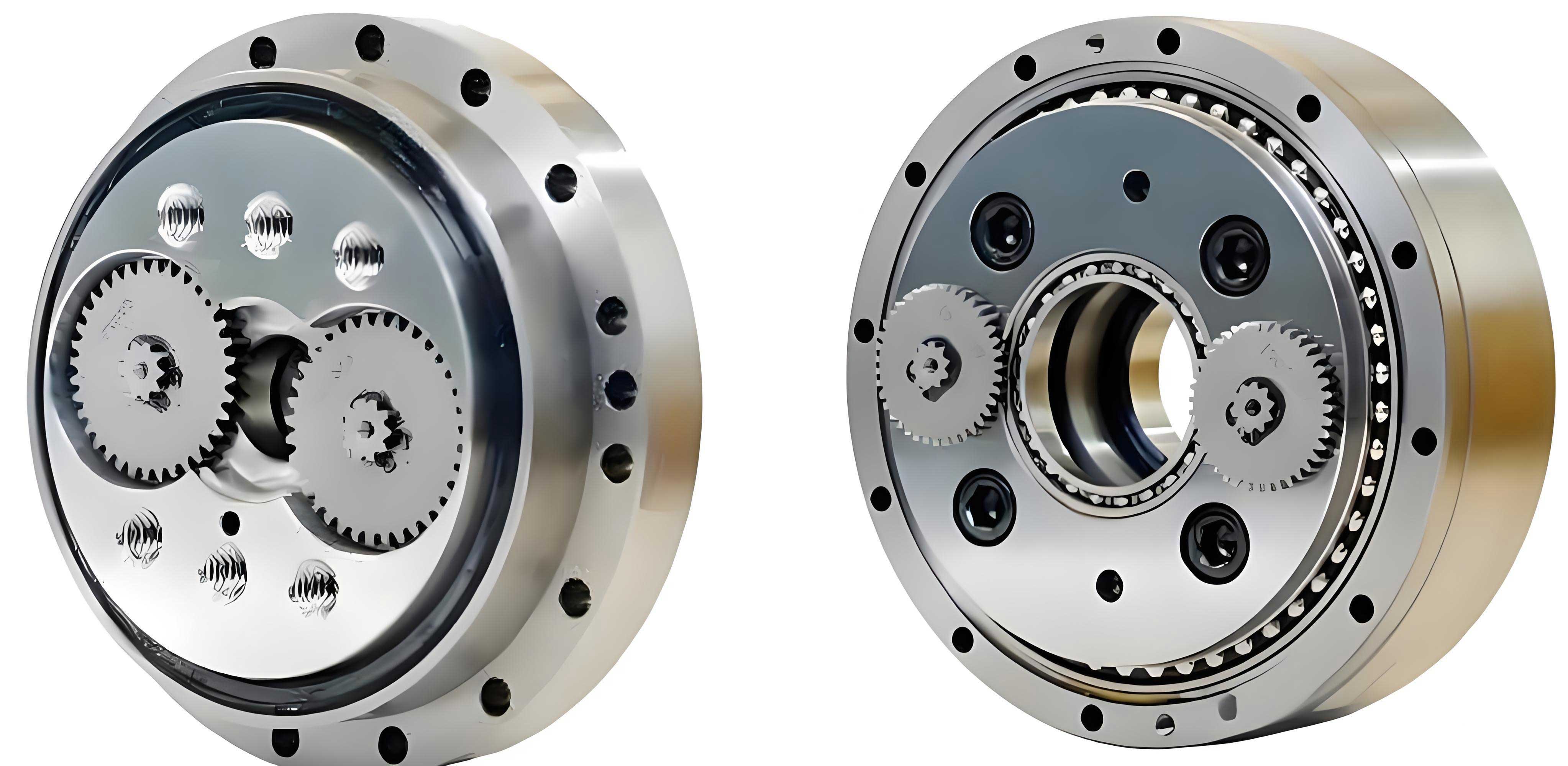
To generate the data necessary for training the surrogate model, a high-fidelity virtual prototype of the RV reducer is essential. We constructed a detailed 3D model, incorporating realistic material properties for critical components, as listed in Table 2. To account for deformations under load—a significant factor for the rotational transmission error in an RV reducer—key load-bearing parts like the crankshafts, cycloid gears, and pins were converted into flexible bodies using finite element analysis. These flexible components were then integrated into a multi-body dynamics model within a commercial simulation environment, creating a rigid-flexible coupled virtual prototype. This model was rigorously validated against physical test bench measurements for several assembled RV reducers. The correlation between simulation results and experimental data was within an acceptable margin of error (under 5%), confirming the virtual prototype’s reliability for generating accurate rotational transmission error data to train our Kriging model.
| Component | Material | Elastic Modulus (GPa) | Density (kg/m³) | Poisson’s Ratio |
|---|---|---|---|---|
| Input Shaft | 15CrMo | 212 | 7880 | 0.284 |
| Planet Gear | 38CrMoAl | 211 | 7850 | 0.277 |
| Crankshaft | 20CrMnMo | 219 | 7830 | 0.300 |
| Cycloid Gear | 20CrMnMo | 207 | 7870 | 0.254 |
| Pin | GCr15 | 219 | 7830 | 0.300 |
| Pin Housing | QT500-7 | 209 | 7890 | 0.269 |
The core of our methodology is the construction of a Kriging surrogate model. The Kriging model is particularly suited for this task concerning the RV reducer because it provides not only a prediction but also an estimate of the prediction error, enabling intelligent adaptive sampling. The model expresses the predicted rotational transmission error y(x) at any point x in the five-dimensional parameter space as:
$$ y(\mathbf{x}) = \mathbf{f}^T(\mathbf{x})\boldsymbol{\beta} + \mathbf{r}^T(\mathbf{x})\boldsymbol{\gamma} $$
Here, $\mathbf{f}^T(\mathbf{x})\boldsymbol{\beta}$ is a global polynomial regression model, and $\mathbf{r}^T(\mathbf{x})\boldsymbol{\gamma}$ is a localized deviation modeled as a Gaussian stochastic process. $\mathbf{x} = [\delta_{rrp}, \delta_{rp}, \delta_{a}, \Delta_{rrp}, \Delta_{rp}]$ is the input vector. The correlation between samples is defined by a Gaussian kernel:
$$ R(\mathbf{x}_i, \mathbf{x}_j) = \exp\left[-\sum_{l=1}^{5} \theta_l (x_i^{(l)} – x_j^{(l)})^2\right] $$
where $\theta_l$ are the correlation parameters to be determined.
Our modeling process began with design of experiments. We employed an Optimal Latin Hypercube Sampling (OLHS) strategy to generate 50 initial sample points within the normalized five-dimensional tolerance space. For each sample point, defined by a specific combination of the five RV reducer parameters, we executed the validated virtual prototype simulation to obtain the corresponding rotational transmission error value. This created our initial training dataset of 50 input-output pairs. An initial Kriging model was fitted to this data. However, the accuracy of this initial model was insufficient for precise selective assembly of the RV reducer, as indicated by relatively high error metrics like Root Mean Square Error (RMSE).
To refine the model efficiently, we implemented an iterative “double-point” infill strategy. In each iteration, two new sample points were selected and added to the training set based on distinct criteria aimed at improving both global and local model accuracy for the RV reducer. The first point was chosen to maximize the Expected Improvement (EI) function, which balances exploration of regions with high prediction uncertainty and exploitation of regions potentially yielding a lower error:
$$ E[I(\mathbf{x})] = (y_{min} – \hat{y}(\mathbf{x})) \Phi\left(\frac{y_{min} – \hat{y}(\mathbf{x})}{s(\mathbf{x})}\right) + s(\mathbf{x}) \phi\left(\frac{y_{min} – \hat{y}(\mathbf{x})}{s(\mathbf{x})}\right) $$
where $y_{min}$ is the current best (minimum) observed error, $\hat{y}(\mathbf{x})$ is the Kriging prediction, $s(\mathbf{x})$ is the predicted standard error, and $\Phi$ and $\phi$ are the standard normal cumulative distribution and probability density functions, respectively. The second point was selected to minimize the predictor’s variance ($MP$ criterion), directly targeting regions where the model is most uncertain about the RV reducer’s behavior:
$$ \mathbf{x}_{MP} = \arg \min [s^2(\mathbf{x})] $$
Finding the global optimum of these nonlinear, multi-modal infill criteria within the RV reducer’s parameter space is computationally challenging. We accelerated this search using the Particle Swarm Optimization (PSO) algorithm. The position and velocity of each particle i at iteration t are updated as:
$$ \begin{aligned} v_i^{(l)}(t+1) &= \omega v_i^{(l)}(t) + c_1 r_1 (p_i^{(l)}(t) – x_i^{(l)}(t)) + c_2 r_2 (g^{(l)}(t) – x_i^{(l)}(t)) \\ x_i^{(l)}(t+1) &= x_i^{(l)}(t) + v_i^{(l)}(t+1) \end{aligned} $$
where $\omega$ is the inertia weight, $c_1$ and $c_2$ are learning factors, $r_1$ and $r_2$ are random numbers, $p_i$ is the particle’s best position, and $g$ is the swarm’s best position.
This infill loop—PSO-based search for EI and MP points, simulation of the RV reducer virtual prototype at these new points, and re-fitting of the Kriging model—was repeated. After 54 infill iterations (adding 108 new samples to the initial 50, resulting in 158 total training points), the model’s accuracy converged to a satisfactory level. The final model parameters and a dramatic improvement in accuracy metrics are shown in Tables 3 and 4. The final model provides a comprehensive, explicit functional relationship mapping the five key RV reducer manufacturing parameters directly to the predicted rotational transmission error.
| Parameter Type | Symbol | Representative Values |
|---|---|---|
| Correlation Parameters | θ | θ1=39.036, θ2=50.000, θ3=28.558, θ4=25.786, θ5=50.000 |
| Regression Coefficients | β | β1=0.668, β2=0.371, β3=-0.429, β4=0.829, β5=0.414, … |
| Accuracy Metric | Initial Model | Final Model |
|---|---|---|
| Root Mean Square Error (RMSE) | 3.7288 | 0.6350 |
| Normalized Max Absolute Error (NMAE) | 0.1500 | 0.0298 |
The ultimate validation of our proposed Kriging model for the RV reducer lies in its performance compared to both the physical prototype and the virtual prototype it intends to surrogate. We conducted a test using three distinct sets of physically measured RV reducer components. For each set, we measured the five key parameters, assembled the physical RV reducer, and measured its rotational transmission error on a test bench. We also performed a full virtual prototype simulation for each set. Finally, we simply plugged the five measured parameter values into our finalized Kriging model to obtain an instantaneous prediction. The results, including the critical time factor, are presented in Table 5.
| Method | Avg. Time per Prediction | Rotational Transmission Error [arcmin] (Set 1 / Set 2 / Set 3) | Avg. Error vs. Physical Test |
|---|---|---|---|
| Physical Test Bench | ~12.5 hours | 1.455 / 1.657 / 1.290 | Baseline |
| Virtual Prototype Simulation | ~1.5 hours | 1.427 / 1.641 / 1.279 | ~1.9% |
| Kriging Model Prediction | ~10 seconds | 1.422 / 1.648 / 1.270 | ~2.1% |
The results are conclusive. The Kriging model achieves prediction accuracy for the RV reducer’s rotational transmission error that is virtually equivalent to the high-fidelity virtual prototype, with an average deviation from physical tests of around 2.1%. However, it accomplishes this not in hours, but in mere seconds. This several-orders-of-magnitude reduction in prediction time transforms the feasibility of selective assembly for the RV reducer in an industrial setting. Our developed Kriging model effectively acts as a real-time performance calculator, allowing manufacturers to instantly evaluate the expected quality of an RV reducer assembly from measured part dimensions before any physical assembly takes place.
In conclusion, our research successfully develops and validates a highly efficient and accurate data-driven prediction method for the rotational transmission error of RV reducers, specifically the RV-40E type. By strategically sampling the parameter space, leveraging a validated virtual prototype for data generation, and employing an adaptive Kriging modeling approach enhanced by a dual-point infill strategy and PSO optimization, we have created a surrogate model that captures the complex, coupled effects of multiple manufacturing tolerances. This model bridges the gap between high-accuracy simulation and the high-speed requirements of industrial practice. It empowers manufacturers to implement effective selective assembly strategies for RV reducers, thereby overcoming limitations in machining precision and significantly improving batch qualification rates and final product quality. Future work could focus on integrating a broader set of influencing factors, such as bearing clearance or thermal effects, into the model framework to further enhance its generality and predictive power for the next generation of high-precision RV reducers.