
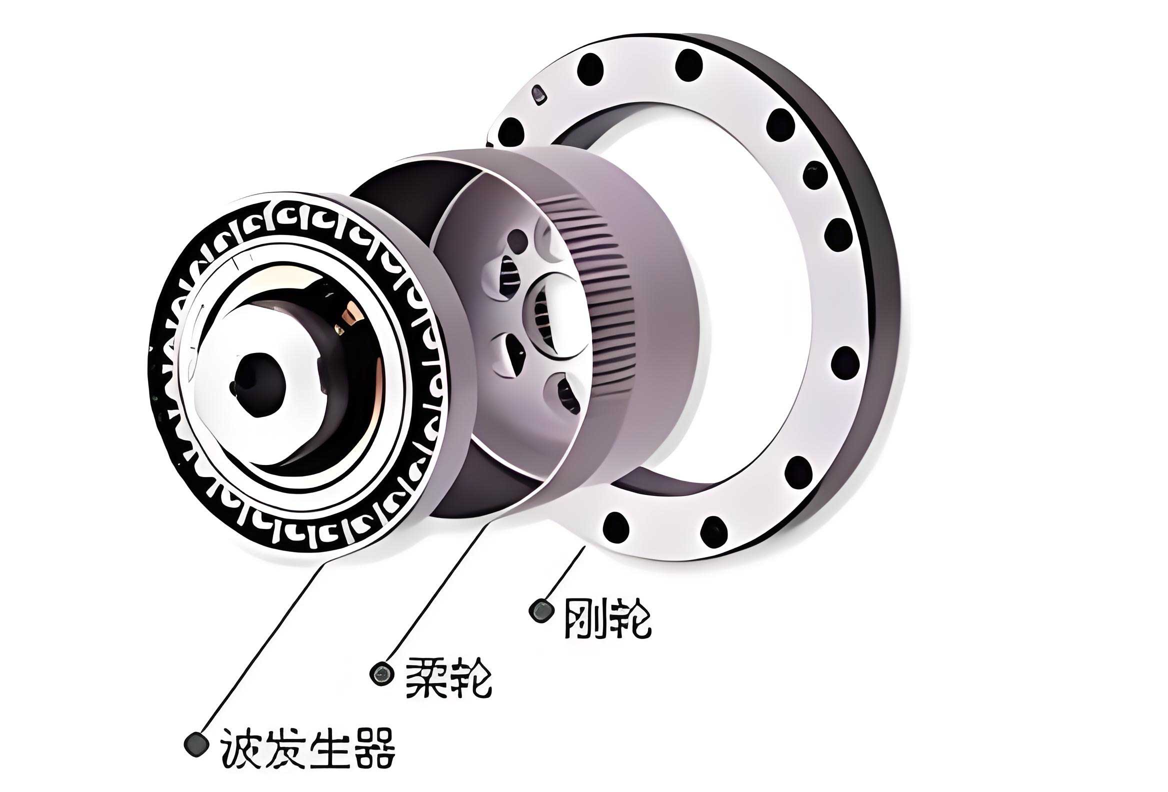
In my pursuit of enhancing the precision and reliability of complex mechanical devices, I have focused on the critical component within their drivetrains: the strain wave gear system. Found in the joints of space manipulators and the pointing mechanisms of spacecraft solar arrays, the performance of these high-ratio reduction devices directly dictates the system’s overall accuracy. At its core, a strain wave gear operates on the principle of elastic deformation. The system typically consists of three primary elements: a rigid Circular Spline (CS), a flexible Flexspline (FS), and a Wave Generator (WG). The WG, often an elliptical bearing or cam, deforms the FS so that its external teeth engage with the internal teeth of the CS at two diametrically opposite regions. As the WG rotates, the elastic wave propagates through the FS, causing a slow, relative rotation between the FS and CS. This unique operating principle, while enabling exceptional advantages like high reduction ratios, compactness, and zero-backlash, also introduces complex, non-linear dynamic behaviors. These behaviors—kinematic error, friction, non-linear stiffness, and hysteresis—severely degrade transmission performance, leading to positional inaccuracies, velocity fluctuations, and energy losses. Therefore, achieving an accurate dynamic model of the strain wave gear transmission is not merely an academic exercise but a fundamental requirement for advancing high-precision robotics and aerospace mechanisms.
The fundamental challenge in modeling stems from the coupling between flexibility and friction inherent to the strain wave gear mechanism. Early research often simplified these phenomena, treating kinematic error as a purely periodic signal and employing static friction models while ignoring hysteresis. With advances in computational power and tribological theory, our understanding has deepened. We now recognize that the dynamic behavior is a result of intricate interactions between component compliance, time-varying meshing conditions, and distributed friction across multiple contact interfaces. This article synthesizes my perspective on the key dynamic behaviors observed in strain wave gear systems and reviews the progression of modeling approaches developed to capture them, highlighting their structures, characteristics, and applicable domains.
Analysis of Key Dynamic Behaviors in Strain Wave Gears
1. Kinematic Error
Kinematic error, defined as the deviation between the ideal and actual output angular position for a given input, is a primary source of inaccuracy. In my analysis, I define it mathematically for a system with reduction ratio $N$ as:
$$ \theta_e = – \frac{\theta_i}{N} – \theta_o $$
where $\theta_i$ is the input displacement and $\theta_o$ is the measured output displacement.
The error signal is not monolithic; it is a superposition of distinct components. The dominant component is a periodic error with a frequency twice that of the wave generator’s rotation ($2f_{WG}$). This primarily originates from manufacturing and assembly imperfections, such as eccentricity of the circular spline or deviations in tooth profile. A simplified mechanism is illustrated below: as the elliptical wave generator rotates, the depth of mesh engagement at the two major axis points ($h_A$ and $h_B$) varies cyclically, leading to a periodic lead/lag in the output.
Superimposed on this periodic error is a high-frequency, stochastic component. I attribute this to the system’s inherent compliance. Under low load conditions, where the overall torsional stiffness is minimal, micro-slip and relative motion can occur between the wave generator and the flexspline. These micro-motions, driven by the high input speed and the non-linear stiffness, introduce random vibrations that manifest as high-frequency noise in the kinematic error signal.
The factors influencing kinematic error are multifaceted and its impact is significant:
- Load: Increasing torque generally reduces the amplitude of kinematic error by stiffening the mesh.
- Speed: Higher input speeds amplify the high-frequency stochastic component.
- Assembly: The depth of insertion of the wave generator into the flexspline inversely affects error magnitude.
The consequences are twofold: it creates a static positional offset and acts as an excitation source for torsional vibrations, which can lead to severe speed ripple at resonant conditions.
2. Friction
Friction within a strain wave gear is a major source of energy loss and a key contributor to hysteresis. In my examination, I identify three primary sources:
- Wave Generator/Flexspline Interface: Friction between the WG bearing outer race and the inner wall of the FS.
- Tooth Meshing Interface: Friction between the engaging teeth of the FS and CS.
- Output Bearing Interface: Friction in the support bearings of the output shaft.
For modeling system-level dynamics, the first two sources are critical. The friction torque exhibits a complex relationship with both input speed and position. Experimentally, I have observed that friction torque often increases with speed at very low velocities (rising static friction or Stribeck effect), then transitions to a velocity-weakening regime before settling into a more linear, viscous-like behavior at higher speeds. Furthermore, it often contains a periodic component synchronized with the WG rotation, reflecting the cyclic variation in contact conditions.
3. Non-Linear Stiffness and Hysteresis
The torsional stiffness of a strain wave gear is decidedly non-linear. When the transmitted torque $T$ is plotted against the angular deformation $\theta$ (where $\theta = \theta_{output} + \theta_{input}/N$), the curve exhibits two hallmark features: stiffness hardening and hysteresis.
Stiffness Hardening: The effective stiffness $k = dT/d\theta$ increases with applied torque. This is a direct consequence of the system’s compliance, primarily from the flexspline’s bending and the wave generator bearing’s deflection. As load increases, the teeth engage more fully and the flexspline’s diaphragm stretches, leading to a progressive stiffening of the transmission path.
Hysteresis: When the torque is cycled from zero to a positive maximum, back to zero, and then to a negative maximum, the torque-deformation path forms a loop. The loading and unloading curves do not coincide. This hysteresis loop represents energy dissipation per cycle. In my view, this is not solely due to flexibility but is a coupled effect of flexibility and friction. The non-linear stiffness defines the backbone of the curve, while friction, particularly pre-sliding micro-displacement and sliding friction in the meshing zones, creates the width and shape of the hysteresis loop.
The consequences are critical for control: hysteresis leads to a loss of positional accuracy as the output position becomes dependent on the torque history, not just its instantaneous value. It also complicates the system’s energy storage and release characteristics during dynamic operation.
Progression of Dynamic Models for Strain Wave Gears
The evolution of models mirrors our deepening understanding of these coupled phenomena. Below, I categorize and discuss the primary modeling approaches.
1. Kinematic Error Models
These models aim to describe the functional relationship $\theta_e = f(\theta_i, \dot{\theta}_i, T, …)$.
a) Trigonometric (Periodic) Model:
This is the simplest approach, capturing only the dominant periodic error. It models the error as a sum of harmonic functions:
$$ \theta_e(t) = \sum_{n=1}^{N} A_n \sin(B_n \theta_i(t) + \phi_n) $$
where $A_n$, $B_n$, and $\phi_n$ are amplitude, frequency multiplier, and phase for the $n^{th}$ harmonic, identifiable via spectral analysis of experimental data. Its strength is simplicity and ease of parameter identification under quasi-static conditions. Its major limitation is the inability to capture the speed-dependent stochastic error or the influence of load.
b) Lagrangian (Compliance-Dependent) Model:
This more advanced framework incorporates system dynamics. I model the strain wave gear as a two-degree-of-freedom system with generalized coordinates $\theta_i$ and $\theta_o$. The kinetic energy ($E$), potential energy ($V$ from the non-linear stiffness), and Rayleigh dissipation function ($\Psi$ for friction) are formulated. The potential energy integral inherently links the kinematic error’s stochastic component $\theta_{e,stiff}$ to the torsional deformation:
$$ \theta_e = -\frac{\theta_i}{N} – \theta_o = \theta_{e,cyc} + \theta_{e,stiff} $$
$$ V = \int_{0}^{\theta_o + \theta_i/N + \theta_{e,cyc}} T(\theta) d\theta $$
Applying Lagrange’s equation yields coupled differential equations that can simulate the dynamic interaction between compliance, excitation, and the resulting high-frequency error. This model is powerful for high-fidelity simulation but requires solving complex equations and accurate knowledge of stiffness and damping parameters.
2. Friction Models
Moving beyond simple Coulomb+viscous models is essential for strain wave gear dynamics.
Dynamic LuGre Friction Model:
This model has been successfully adapted for strain wave gears. It conceptualizes friction interfaces as contacting bristles. The average bristle deflection $z$ is a state variable:
$$ \frac{dz}{dt} = \dot{\theta}_i – \frac{|\dot{\theta}_i|}{g(\dot{\theta}_i)} z $$
$$ g(\dot{\theta}_i) = \frac{1}{\sigma_0} \left[ F_c + (F_s – F_c) e^{-(\dot{\theta}_i/\omega_s)^2} \right] $$
where $F_c$ is Coulomb friction, $F_s$ is stiction torque, $\omega_s$ is the Stribeck velocity, and $\sigma_0$ is the bristle stiffness. The total friction torque $T_{fr}$ is then:
$$ T_{fr} = \underbrace{\sigma_0 z + \sigma_1 \dot{z} + \sigma_2 \dot{\theta}_i}_{T_{fr,non}} + \underbrace{(A+B\dot{\theta}_i) \cdot f(\theta_i)}_{T_{fr,cyc}} $$
Here, $T_{fr,non}$ captures the rate-dependent non-linear effects (Stribeck, pre-sliding), and $T_{fr,cyc}$ is a periodic component modeling the positional variation of friction, often expressed as a Fourier series in $\theta_i$. This model is comprehensive and suitable for model-based friction compensation in control systems.
3. Non-Linear Stiffness Models
These models describe the steady-state relationship $T = f(\theta)$, ignoring hysteresis.
| Model Type | Mathematical Form | Characteristics & Applicability |
|---|---|---|
| Piecewise Linear | $T = \begin{cases} k_1 \theta, & |\theta| \le \theta_{thr} \\ k_1 \theta + k_2(|\theta|-\theta_{thr}) \cdot sign(\theta), & |\theta| > \theta_{thr} \end{cases}$ | Simple, captures bilinear hardening. Discontinuous derivative at threshold $\theta_{thr}$. Useful for conceptual analysis. |
| Cubic Polynomial | $T = a_1 \theta + a_3 \theta^3$ | Smooth, continuous derivative. Captures progressive hardening effectively. Commonly used in controller design for its simplicity. Cannot describe asymmetric behavior. |
4. Hysteresis Stiffness Models
These are the most comprehensive models, aiming to capture the memory-dependent, history-based torque-deformation relationship $T(t) = f(\theta(t), \text{history of } \theta)$.
a) Memory-Based Model:
This model is founded on the system’s “fading memory” property. The total torque is the sum of a non-linear stiffness function $T_{stiff}(\theta)$ and a friction functional $T_{fri}(t)$:
$$ T(t) = T_{stiff}(\theta(t)) + \int_{0}^{t} \Phi(V_t^s(\theta)) \frac{d\theta(s)}{ds} ds $$
where $V_t^s(\theta)$ is the total variation of $\theta$ on $[s, t]$, and $\Phi(u)$ is a decreasing memory kernel (e.g., $\Phi(u)=Ae^{-\alpha u}$). This leads to a differential equation for $T_{fri}$:
$$ \frac{dT_{fri}}{dt} + \alpha \left|\frac{d\theta}{dt}\right| T_{fri} – A \frac{d\theta}{dt} = 0 $$
This model elegantly captures rate-dependent hysteresis with few parameters ($A$, $\alpha$). However, the assumption of exponentially fading memory may not hold for all strain wave gear interactions.
b) Generalized Maxwell-Slip (GMS) / Iwan-Type Model:
This is a physics-inspired, distributed-element model that I find particularly intuitive for capturing the pinning-depinning behavior in frictional contacts. It represents the interface as a parallel array of $N$ elasto-plastic elements (Jenkins elements). Each element $i$ has a stiffness $k_i$ and a breakaway force $F_{b,i}$. The total torque is:
$$ T(t) = \sum_{i=1}^{N} T_i(t) $$
The state of each element evolves as:
$$ T_i(t) = \begin{cases}
k_i (\theta(t) – \theta_{c,i}), & \text{if } |k_i (\theta(t) – \theta_{c,i})| < F_{b,i} \quad \text{(Stick)} \\
F_{b,i} \cdot sign(\dot{\theta}(t)), & \text{otherwise} \quad \text{(Slip)}
\end{cases} $$
where $\theta_{c,i}$ is the “capture” position where the element last stuck. This model naturally produces hysteresis loops with non-local memory (i.e., the output depends on past extreme inputs, not just the immediate past). It is very accurate but requires identification of a distribution of parameters ($k_i$, $F_{b,i}$), which can be complex.
c) Multi-Compliance Model:
This model explicitly accounts for the flexibility of both the flexspline and the wave generator. I define deformations for both components: $\theta_f$ for the FS and $\theta_w$ for the WG. Their stiffnesses are often modeled as torque-dependent:
$$ K_f = \frac{dT_f}{d\theta_f} = K_{f0} \cdot [1 + (C_f T_f)^2] $$
$$ K_w = \frac{dT_w}{d\theta_w} = K_{w0} \cdot e^{C_w |T_w|} $$
The system deformation $\theta$ is a function of both:
$$ \theta = \theta_f – \frac{\theta_w}{N} = \frac{\arctan(C_f T_f)}{C_f K_{f0}} – \frac{sign(T_w)}{N C_w K_{w0}} (1 – e^{-C_w |T_w|}) $$
where $T_w = -(T_f – T_{fr})/N$. This model provides a clear physical insight into the contribution of different components to the overall compliance and the resulting hysteresis when combined with a friction model $T_{fr}$. It is relatively parsimonious in parameters.
| Hysteresis Model | Core Principle | Advantages | Disadvantages |
|---|---|---|---|
| Memory-Based | Fading memory integral. | Compact form (2-3 parameters), differential equation form. | Assumes specific memory decay; may not capture all hysteresis shapes. |
| Generalized Maxwell-Slip (GMS) | Parallel array of stick-slip elements. | Physically intuitive, captures non-local memory, highly accurate. | Many parameters to identify; computationally more intensive. |
| Multi-Compliance | Separates flexspline and wave generator compliance. | Clear physical interpretation, moderate number of parameters. | Often requires coupling with a separate friction model; may oversimplify contact mechanics. |
Current Challenges and Future Research Directions
Despite significant progress, my work in this field highlights several open challenges that require further investigation:
- Mechanistic Origin of Stochastic Kinematic Error: While Lagrangian models link it to compliance, a precise, physics-based model connecting specific flexspline vibration modes or wave generator bearing kinematics to the high-frequency error spectrum is still needed. Future research should employ detailed multi-body dynamics or finite element analysis of the meshing process to uncover these mechanisms.
- Coupled Friction-Flexibility Mechanisms: The exact contribution of different friction sources (tooth mesh vs. WG/FS interface) to the overall hysteresis loop shape under varying loads and speeds is not fully quantified. Advanced tribological models that incorporate mixed lubrication regimes, especially for the WG bearing, need to be integrated into system-level dynamic models of the strain wave gear.
- Unified High-Fidelity Modeling Framework: There is a need for a comprehensive yet computationally tractable model that seamlessly integrates a non-local memory hysteresis model (like GMS) for friction, a non-linear stiffness model for the flexspline and wave generator, and a kinematic error model that includes both deterministic and stochastic components. This framework should be valid across the full operational envelope (speed, torque, temperature).
- Model-Based Control and Compensation: Translating these advanced dynamic models into real-time, robust control algorithms for ultra-precision applications remains a practical challenge. Research into adaptive and learning-based control that can identify and compensate for the time-varying parameters of these non-linear models is a critical next step.
In conclusion, the journey of dynamic modeling for strain wave gear systems has evolved from simplistic linear approximations to sophisticated non-linear, hysteresis-aware frameworks. The choice of model depends critically on the application’s requirements: precision of simulation, need for real-time compensation, or depth of physical insight. The persistent challenges lie in deepening our mechanistic understanding of the micro-scale interactions and effectively integrating this knowledge into robust, high-fidelity models that empower the next generation of precision mechanical systems.