
In the realm of power transmission systems, helical gears are paramount components, extensively employed in demanding applications across aerospace, automotive, and maritime industries due to their superior load-carrying capacity and smoother, quieter operation compared to spur gears. The dynamic performance, service life, safety, and reliability of these systems are profoundly influenced by the inherent characteristics of the helical gears within them. A critical internal excitation governing the vibrational signature of a gear transmission system is the Time-Varying Meshing Stiffness (TVMS). This parameter fluctuates as the number of teeth in contact changes and as the contact position moves along the tooth profile during rotation. Consequently, the accurate calculation of TVMS is a cornerstone for dynamic modeling, noise-vibration-harshness (NVH) prediction, and condition monitoring of gear systems.
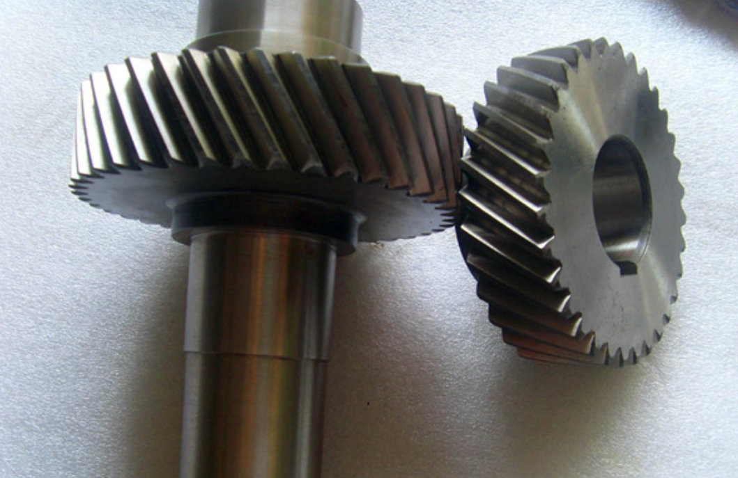
While significant research has been devoted to TVMS calculation for spur gears using analytical methods like the potential energy method, the analysis for helical gears presents additional complexity. The primary challenge stems from the inclined tooth trace, which results in gradual engagement and disengagement along the face width. Traditional analytical approaches often simplify this by employing the “slice method,” where the helical gear is discretized into a series of thin, independent spur gear slices along its axis. The total mesh stiffness is then assumed to be the sum of the stiffnesses of the individual slices that are in contact at any given time. However, this conventional uncoupled slice model overlooks a crucial mechanical phenomenon: the structural coupling between adjacent slices. A slice experiencing direct loading will deform, but this deformation is resisted not only by its own stiffness but also by the adjacent, non-loaded slices through the continuous gear body. This coupling effect effectively stiffens the gear tooth beyond what the simple sum of independent slices would predict. Ignoring this coupling, particularly in transition zones where contact is partial, can lead to underestimation of the mesh stiffness.
This article addresses this gap by proposing an enhanced analytical model for calculating the TVMS of helical gears based on a coupled slice theory. The model rigorously accounts for the interaction between slices, leading to a more accurate representation of the gear tooth’s true structural response. We begin by detailing the fundamental stiffness models for a single gear tooth, followed by the formulation of the novel slice coupling theory. A numerical solution scheme is then presented. Finally, the proposed model is validated against a detailed 3D Finite Element Analysis (FEA) model, and its results are critically compared with those from the traditional uncoupled slice method.
Fundamental Stiffness Components of a Gear Tooth
Before delving into the coupling of slices for helical gears, it is essential to define the basic stiffness components of a single gear tooth, modeled as a non-uniform cantilever beam rooted at the gear base. For a spur gear slice (which represents a thin section of a helical gear), the total tooth compliance comprises contributions from bending, shear, axial compression, and the foundation (or fillet) region. The Hertzian contact deformation between two mating teeth is treated separately.
Using the potential energy method and referring to the beam model, the stiffness values for bending ($$k_b$$), shear ($$k_s$$), and axial compression ($$k_a$$) for a single tooth under load at point $$F$$ are given by the following integrals along the tooth profile:
$$ \frac{1}{k_b} = \int_{\phi_t}^{\pi/2} \frac{[\cos\phi_1 (y_{\phi_1} – y_1) – x_{\phi_1} \sin\phi_1]^2}{EI_{y1}} \frac{dy_1}{d\gamma} d\gamma + \int_{\phi_1}^{\tau_C} \frac{[\cos\phi_1 (y_{\phi_1} – y_2) – x_{\phi_1} \sin\phi_1]^2}{EI_{y2}} \frac{dy_2}{d\tau} d\tau $$
$$ \frac{1}{k_s} = \int_{\phi_t}^{\pi/2} \frac{1.2\cos^2\phi_1}{GA_{y1}} \frac{dy_1}{d\gamma} d\gamma + \int_{\phi_1}^{\tau_C} \frac{1.2\cos^2\phi_1}{GA_{y2}} \frac{dy_2}{d\tau} d\tau $$
$$ \frac{1}{k_a} = \int_{\phi_t}^{\pi/2} \frac{\sin^2\phi_1}{EA_{y1}} \frac{dy_1}{d\gamma} d\gamma + \int_{\phi_1}^{\tau_C} \frac{\sin^2\phi_1}{EA_{y2}} \frac{dy_2}{d\tau} d\tau $$
Where:
– $$E$$, $$G$$, and $$\nu$$ are the material’s Young’s modulus, shear modulus, and Poisson’s ratio, respectively.
– $$I_{y1}, A_{y1}$$ and $$I_{y2}, A_{y2}$$ are the area moment of inertia and cross-sectional area at points on the trochoidal fillet and involute profile segments, respectively.
– $$y_{\phi_1}$$ is the horizontal distance from the load application point to the tooth root.
– $$\phi_1$$ is the pressure angle at the load point.
– Other geometric parameters ($$y_1, y_2, x_{\phi_1}, \phi_t, \tau_C$$) define the tooth geometry and integration limits.
The combined tooth stiffness ($$k_t$$) from these three deflections, acting in series, for a slice of thickness $$\Delta l$$ is:
$$ k_t = \frac{1}{\frac{1}{k_b} + \frac{1}{k_s} + \frac{1}{k_a}} $$
The Hertzian contact stiffness for two parallel cylinders, modeling the contact between two slices, is:
$$ k_h = \frac{\pi E \Delta l}{4(1 – \nu^2)} $$
Furthermore, the deflection of the gear body (foundation) under tooth load is significant. For a single tooth pair engagement, the foundation stiffness ($$k_f$$) can be approximated by a semi-empirical formula:
$$ \frac{1}{k_f} = \frac{\cos^2\phi_1}{E \Delta l} \times \left[ L^* \left( \frac{u_f}{S_f} \right)^2 + M^* \left( \frac{u_f}{S_f} \right) + P^* \left(1 + Q^* \tan^2\phi_1 \right) \right] $$
Where $$u_f$$ and $$S_f$$ are geometric parameters related to the distance from the root circle to the gear bore. The coefficients $$L^*$$, $$M^*$$, $$P^*$$, and $$Q^*$$ are polynomial functions of the normalized rim thickness $$h_f = r_f / r_{int}$$ and the angle $$\theta_f$$ subtended by the tooth base. They are calculated as:
$$ X_i^*(h_f, \theta_f) = A_i / \theta_f^2 + B_i h_f^2 + C_i h_f / \theta_f + D_i / \theta_f + E_i h_f + F_i $$
Where $$X_i^*$$ represents any of the four coefficients. The constants $$A_i$$ through $$F_i$$ are tabulated below:
| Coefficient | $$A_i$$ | $$B_i$$ | $$C_i$$ | $$D_i$$ | $$E_i$$ | $$F_i$$ |
|---|---|---|---|---|---|---|
| $$L^*$$ | -5.574E-5 | -1.9986E-3 | -2.3015E-4 | 4.7702E-3 | 0.0271 | 6.8045 |
| $$M^*$$ | 60.111E-5 | 28.1E-3 | -83.431E-4 | -9.9256E-3 | 0.1624 | 0.9086 |
| $$P^*$$ | -50.952E-5 | 185.5E-3 | 0.0538E-4 | 53.3E-3 | 0.2895 | 0.9236 |
| $$Q^*$$ | -6.2042E-5 | 9.0889E-3 | -4.0964E-4 | 7.8297E-3 | -0.1472 | 0.6904 |
In multi-tooth engagement regions, the simple summation of individual foundation stiffnesses is inaccurate due to mutual constraint. Therefore, a modified combined foundation stiffness ($$k_{tf}$$) for the gear pair is used:
$$ k_{tf} = 1 / \left( \frac{1}{\lambda_p k_{fp}} + \frac{1}{\lambda_g k_{fg}} \right) $$
Here, $$k_{fp}$$ and $$k_{fg}$$ are the single-tooth foundation stiffnesses for the pinion and gear, respectively. $$\lambda_p$$ and $$\lambda_g$$ are correction factors ($$\lambda \ge 1$$) that account for the stiffening effect in multi-tooth contact, often determined via finite element analysis. For single-tooth contact, $$\lambda = 1$$.
Coupled Slice Theory for Helical Gears
The engagement of helical gears is characterized by a sloping contact line that moves across the face width. At any instant, the contact region is a band spanning only a portion of the total face width. This means some slices are in full contact, some are partially engaged, and others are completely disengaged. In the traditional uncoupled model, only the stiffness of the slices in the instantaneous contact zone contributes to the total mesh stiffness. This neglects the fact that the gear tooth is a continuous three-dimensional elastic body. A loaded slice will tend to deflect, but this deflection is constrained by the adjacent material of the unloaded slices, which act as a distributed elastic support. This inter-slice coupling effect increases the overall effective stiffness of the tooth.
To model this, we propose a coupled slice theory. The helical gear tooth is discretized into $$N$$ slices of thickness $$\Delta l$$. Each slice has an associated tooth stiffness ($$k_{t,i}$$) calculated as per the previous section. Adjacent slices are connected by coupling springs that represent the resistance to relative deflection between slices, primarily due to the bending and shear of the “web” of material between them. The stiffness of this coupling spring between slice $$i$$ and $$i+1$$ is postulated to be proportional to the average tooth stiffness of the two slices and inversely related to the square of the slice thickness, scaled by the module $$m$$:
$$ k_{c,i(i+1)} = C_c \cdot \left( \frac{k_{t,i} + k_{t,i+1}}{2} \right) \left( \frac{m}{\Delta l} \right)^2 $$
Where $$C_c$$ is a coupling factor. For the continuum body of a helical gear, this factor is taken as $$C_c = 1$$.
Consider a tooth loaded by a set of slice forces $$F_i$$, resulting in slice deflections $$\delta_{t,i}$$. The force equilibrium for an internal slice $$i$$ is governed by the interaction with its neighbors:
$$ -k_{c,(i-1)i}(\delta_{t,i-1} – \delta_{t,i}) + k_{t,i}\delta_{t,i} + k_{c,i(i+1)}(\delta_{t,i} – \delta_{t,i+1}) = F_i $$
For the first and last slice, the equations are:
$$ k_{t,1}\delta_{t,1} + k_{c,12}(\delta_{t,1} – \delta_{t,2}) = F_1 $$
$$ -k_{c,(N-1)N}(\delta_{t,N-1} – \delta_{t,N}) + k_{t,N}\delta_{t,N} = F_N $$
The total force on the tooth is the sum of the slice forces: $$F = \sum_{i=1}^{N} F_i$$.
In the context of mesh stiffness calculation, a key scenario arises when only some slices are in direct contact (transmitting $$F_i > 0$$), while others are not ($$F_i = 0$$). For a non-contact slice $$j$$ located between two loaded or constrained regions, its deflection is not zero but is induced through the coupling springs. This induced deflection can be related to the deflection of an adjacent slice via a deflection transfer coefficient $$\Gamma$$:
$$ \delta_{t, (i+1)} = \Gamma_{i(i+1)} \delta_{t, i} \quad \text{(for a non-contact slice)} $$
The transfer coefficient $$\Gamma_{i(i+1)}$$ can be derived recursively from the system’s equilibrium equations, considering the boundary conditions of the non-contact region.
For a mating gear pair, the total deformation at a contacting slice $$i$$ is the sum of the deflections of the driving tooth ($$\delta_{p,i}$$), driven tooth ($$\delta_{g,i}$$), and the Hertzian contact ($$\delta_{h,i}$$):
$$ \delta_{p,i} + \delta_{g,i} + \delta_{h,i} = \delta_i $$
The force equilibrium gives: $$k_{p,i}\delta_{p,i} = k_{g,i}\delta_{g,i} = k_{h,i}\delta_{h,i} = F_i$$. Therefore, the total mesh deformation at slice $$i$$ can be expressed in terms of, for example, the pinion slice deflection:
$$ \delta_i = \frac{k_{p,i}k_{h,i} + k_{g,i}k_{h,i} + k_{p,i}k_{g,i}}{k_{g,i}k_{h,i}} \delta_{p,i} $$
Finally, the total mesh stiffness ($$k_{tt}$$) for the tooth pair is the ratio of total force to total effective deflection. Incorporating the foundation stiffness ($$k_{tf}$$) in series yields the overall system mesh stiffness ($$k$$):
$$ k = \frac{1}{\frac{1}{k_{tt}} + \frac{1}{k_{tf}}}} $$
Numerical Solution Procedure for TVMS
Calculating the TVMS for helical gears using the coupled theory requires a numerical iterative approach due to the interdependent slice deflections, especially when partial contact occurs. The procedure is as follows:
- Input Parameters: Define gear geometry (number of teeth $$z$$, module $$m$$, face width $$B$$, helix angle $$\beta$$, pressure angle $$\alpha$$), material properties ($$E$$, $$G$$, $$\nu$$), and applied torque $$T$$.
- Discretization and Initialization: Discretize the face width into $$N$$ slices (e.g., $$N=50$$). Determine the initial meshing position of the helical gear pair. For each rotational position (mesh phase), identify which slices are in contact based on the lead of the helix.
- Stiffness Calculation: For each slice $$i$$, calculate its individual tooth stiffness components ($$k_{b,i}, k_{s,i}, k_{a,i}$$) to get $$k_{t,i}$$. Compute the inter-slice coupling stiffness $$k_{c,i(i+1)}$$ and the foundation stiffness $$k_{tf}$$.
- Iterative Solution for Deflection:
- Assume an initial total mesh deflection $$\delta$$ for the engaged portion.
- Distribute this deflection among the contacting slices, estimating initial $$\delta_{p,i}$$ values.
- Using the system of equilibrium equations (including coupling springs) and the relations for non-contact slices, solve for the updated slice forces $$F_i$$ and the corresponding total mesh force $$F_m = \sum F_i$$.
- Compare $$F_m$$ with the known external load $$F$$ derived from the applied torque.
- If $$|F – F_m| > F_{\epsilon}$$ (where $$F_{\epsilon}$$ is a small tolerance, e.g., 1 N), update the assumed total deflection $$\delta$$ and repeat the force calculation.
- If $$|F – F_m| \le F_{\epsilon}$$, the equilibrium state is found. The corresponding deflection $$\delta$$ and forces $$F_i$$ are final.
- Stiffness Computation: For the converged state, compute the total tooth pair stiffness $$k_{tt} = F / \delta$$. Then, calculate the overall system mesh stiffness $$k$$ using the foundation stiffness in series.
- Time-Varying Calculation: Advance the gear by a small angular increment to the next meshing phase and repeat steps 2-5. Continue until a full mesh cycle (angular period of $$\frac{2\pi}{z}$$) is completed, thus obtaining the TVMS curve.
Model Validation and Comparative Analysis
To validate the proposed coupled slice theory, a case study is performed on a pair of identical steel helical gears. The key parameters are listed in the table below:
| Parameter | Pinion / Gear |
|---|---|
| Number of Teeth, $$z_1 / z_2$$ | 35 / 35 |
| Module, $$m$$ (mm) | 5 |
| Face Width, $$B$$ (mm) | 16 |
| Pressure Angle, $$\alpha$$ (°) | 20 |
| Helix Angle, $$\beta$$ (°) | 15 |
| Young’s Modulus, $$E$$ (GPa) | 210 |
| Poisson’s Ratio, $$\nu$$ | 0.3 |
| Applied Torque, $$T$$ (N·m) | 200 |
Three models are compared:
1. 3D Finite Element Model (FEM): A high-fidelity nonlinear contact analysis is conducted using solid elements. The mesh is refined at the contact zones. The TVMS is derived from the kinematic relationship between the applied torque and the calculated static angular deflection.
2. Proposed Coupled Slice Model (CSM): Implemented with $$N=50$$ slices, $$C_c=1$$, and foundation correction factor $$\lambda = 1.09$$ (calibrated from FEM).
3. Traditional Uncoupled Slice Model (USM): Implemented with the same discretization but with $$C_c = 0$$, effectively turning off the inter-slice coupling springs.
The resulting TVMS curves over one mesh cycle are plotted together. The mesh cycle for helical gears typically shows two major peaks (double-tooth contact zones) and one lower plateau (single-tooth contact zone), with smooth transitions between them due to the gradual engagement.
The key findings from the comparison are summarized in the following table, which shows the maximum relative error of each analytical method compared to the FEM benchmark in different contact regions:
| Calculation Method | Max Relative Error vs. FEM | Max Relative Error vs. FEM | Max Relative Error vs. FEM |
|---|---|---|---|
| (Single-Tooth Contact Zone) | (Double-Tooth Transition Zone) | (Full Double-Tooth Zone) | |
| Uncoupled Slice Model (USM) | 0.2% | 2.0% | 0.5% |
| Coupled Slice Model (CSM) | 0.5% | 0.7% | 0.6% |
Analysis of Results:
The proposed Coupled Slice Model (CSM) demonstrates excellent agreement with the FEM results across all meshing phases—single-tooth contact, double-tooth transition, and full double-tooth contact—with a maximum discrepancy of only 0.7%. This validates the accuracy of the slice coupling formulation.
The Uncoupled Slice Model (USM) also performs reasonably well in the single-tooth and full double-tooth zones, where the contact region spans most or all of the face width, minimizing the relative impact of coupling. However, its critical weakness is revealed in the double-tooth transition zones. These are the regions where one tooth pair is nearing the end of contact (only a few slices engaged) while another is just beginning contact (also only a few slices engaged). In these phases, a significant portion of the tooth face width is not under direct load. The USM, by ignoring the stiffening effect of these non-contact regions, underestimates the mesh stiffness, leading to a more pronounced error (up to 2.0%). The CSM correctly captures this stiffening effect through the coupling springs, resulting in a TVMS value much closer to the FEM result.
Furthermore, a mesh convergence study was conducted by varying the number of slices $$N$$. The results show that for $$N \ge 50$$, the TVMS curve becomes smooth and converged. Using fewer slices (e.g., $$N=10$$ or $$25$$) leads to noticeable numerical “steps” or “bumps” in the stiffness curve, as the engagement/disengagement of each thick slice causes an abrupt change in the calculated stiffness. Therefore, $$N=50$$ provides an optimal balance between computational efficiency and accuracy for this case.
Conclusion
Accurate modeling of Time-Varying Meshing Stiffness is crucial for the dynamic analysis of helical gear transmission systems. This work has successfully developed and validated an enhanced analytical model based on a novel coupled slice theory. The model advances the traditional slice method by explicitly accounting for the elastic coupling between adjacent slices of the helical gear tooth. This coupling, represented by inter-slice springs, captures the constraining effect that non-loaded portions of the tooth have on the deflection of the loaded portions.
The comparative analysis against a detailed 3D finite element model and the traditional uncoupled approach conclusively demonstrates the superiority of the proposed method. While both slice-based methods are adequate in regions of full-face contact, the coupled slice theory is essential for accurately predicting stiffness in the critical transition zones between single and double tooth contact, where partial face contact occurs. The uncoupled model consistently underestimates stiffness in these regions due to its omission of this fundamental gear body effect.
The presented model offers a computationally efficient and physically accurate alternative to full-scale FE simulations for TVMS calculation in helical gears. It provides a solid foundation for incorporating further complexities such as profile modifications, manufacturing errors, or tooth faults like cracks and spalls into the dynamic analysis of helical gear systems, enabling more reliable design and diagnostics.