
In the realm of agricultural machinery, the operational efficiency and environmental impact of equipment are paramount. A persistent challenge faced in the development of domestic cotton harvesters is the presence of intense vibration and noise emanating from their core working assemblies. This issue is particularly pronounced in the bevel gear transmission system, a critical component responsible for transferring power and motion within the cotton picking head. Historically reliant on imported designs, domestically developed bevel gear systems often exhibit unsatisfactory acoustic performance during operation. The root causes are multifaceted, stemming from dynamic excitations generated by varying numbers of meshing teeth, manufacturing inaccuracies, and impact-induced tooth deformations. These excitations induce random vibrations within the gear pair. This vibration energy is transmitted through the gear shafts to the supporting bearings and ultimately to the entire surface of the bevel gear housing, exciting its structural modes and radiating noise into the environment. Addressing this problem necessitates a deep, predictive understanding of the coupled dynamic behavior encompassing the structural vibrations and the resultant acoustic radiation.
This study presents a comprehensive, simulation-driven methodology for analyzing the multi-field coupled vibration and noise characteristics of a cotton picker’s bevel gear system. The core objective is to establish a virtual prototyping framework that integrates multi-body dynamics, structural dynamics, and acoustics to predict noise radiation at the design stage. The methodology employs a sequential coupling approach, where the output from one analysis serves as the input for the next. The complete transmission system, including gears, shafts, housing, and bearings, is considered as the acoustic boundary element model for noise prediction. The following sections detail the numerical models, solution techniques, and key findings, providing a theoretical foundation for vibration and noise reduction in such mechanical systems.
Research Methodology and Numerical Framework
The analysis follows a structured, multi-step workflow designed to capture the chain of events from gear excitation to sound radiation. The foundational step involves creating a high-fidelity digital model of the entire bevel gear assembly. Subsequent steps focus on extracting its inherent dynamic properties, calculating the operational dynamic loads, simulating its forced vibration response, and finally predicting the radiated noise. The specific research pathway is systematically outlined below.
| Step | Analysis Type | Primary Tool/Theory | Key Output |
|---|---|---|---|
| 1 | 3D Parametric Modeling | CAD Software (e.g., NX) | Digital Twin of the Bevel Gear System |
| 2 | Modal Analysis | Finite Element Method (NASTRAN Solver) | Natural Frequencies and Mode Shapes |
| 3 | Dynamic Load Calculation | Multi-body Dynamics (RecurDyn, Recursive Algorithm) | Time-domain Dynamic Meshing Force |
| 4 | Forced Vibration Response | Transient Dynamic Analysis (NASTRAN) | Nodal Accelerations on Housing Surface |
| 5 | Acoustic Radiation Analysis | Acoustic Boundary Element Method (LMS Virtual.Lab) | Sound Pressure Level Distribution (Noise Cloud Map) |
This integrated approach ensures that the dynamic excitation from the gear contact is faithfully propagated through the structural model to obtain the surface vibration velocities, which act as the essential boundary condition for the acoustic simulation.
Establishing the Numerical Model of the Bevel Gear System
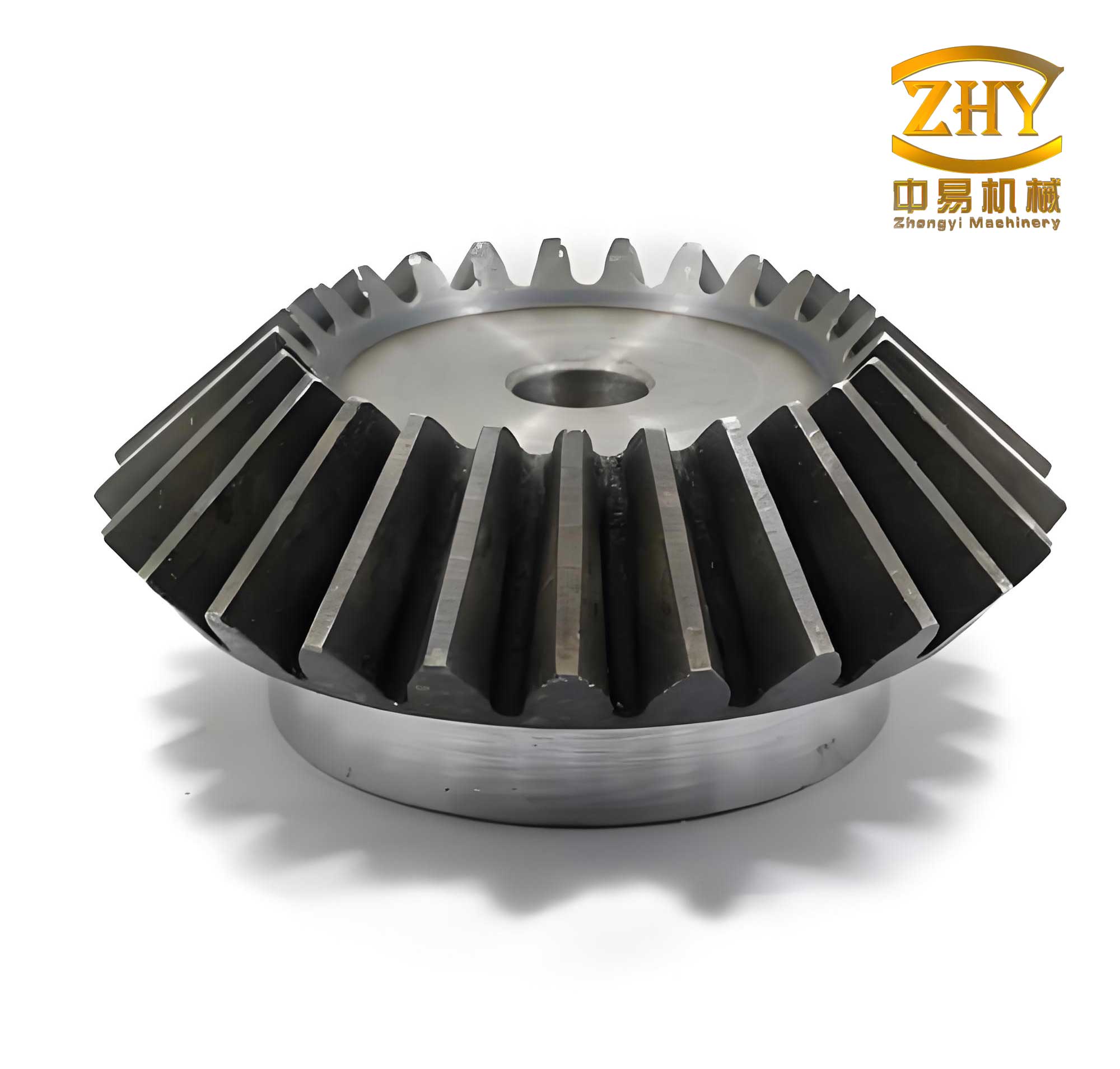
The accuracy of any numerical simulation is contingent upon the fidelity of its underlying geometric model. For this study, a complete digital assembly of the ZM-45 cotton picker’s bevel gear drive was constructed. This model meticulously includes all components that contribute to the system’s dynamic and acoustic behavior: the conjugated bevel gear pair, transmission shafts, the bevel gear housing (gearbox), rolling-element bearings, bearing caps, pulley wheels, and flange plates. Each component is a potential source or transmission path for vibration. The geometric parameters of the bevel gear pair are critical for determining mesh stiffness and excitation characteristics and are summarized in the table below.
| Parameter | Pinion (Driving Gear) | Gear (Driven Gear) |
|---|---|---|
| Number of Teeth (z) | 21 | 29 |
| Module (m) [mm] | 3.75 | |
| Pitch Cone Angle (δ) | 35° 55′ | 54° 5′ |
| Root Cone Angle | 32° 05′ | 50° 15′ |
| Pressure Angle (α) | 20° | |
| Cone Distance (R) [mm] | 108.75 | |
| Pitch Diameter (d) [mm] | 78.75 | 64.134 |
This digital model replaces physical prototypes for virtual experimentation, allowing for efficient and cost-effective investigation of design modifications aimed at noise reduction.
Finite Element Modal Analysis for Inherent Dynamic Characteristics
Understanding the inherent dynamic properties—natural frequencies and mode shapes—of the bevel gear housing and the assembled system is the cornerstone of vibration analysis. These properties determine how the structure will respond to dynamic loads. The modal analysis was performed using the NASTRAN finite element solver, employing the Lanczos algorithm, which is efficient for extracting eigenvalues in large systems. The process flow is standard: import the geometry, define material properties (typically cast iron for the housing and steel for gears/shafts), generate a suitable finite element mesh (combining solid elements for bulky parts and shell elements for thin walls), apply appropriate constraints (simulating bearing supports), and finally solve the eigenvalue problem. The governing equation for undamped free vibration is:
$$ [M]\{\ddot{x}\} + [K]\{x\} = \{0\} $$
Assuming harmonic motion $\{x\} = \{\phi\} e^{j \omega t}$, the equation reduces to the classic eigenvalue problem:
$$ \left( [K] – \omega^2 [M] \right) \{\phi\} = \{0\} $$
where $[M]$ is the global mass matrix, $[K]$ is the global stiffness matrix, $\omega$ is the natural frequency (rad/s), and $\{\phi\}$ is the corresponding mode shape vector. Empirical and simulation experience indicates that the low to medium-frequency modes have the most pronounced influence on vibration and noise radiation. Therefore, the first 20 natural frequencies and their dominant vibration directions for the bevel gear system were extracted and are tabulated below. These results form the basis for subsequent forced response analysis, as excitations near these frequencies can lead to resonance and amplified vibration.
| Mode Order | Natural Frequency (Hz) | Peak Amplitude (mm) | Primary Vibration Direction |
|---|---|---|---|
| 1 | 3.529e+2 | 0.618 | X-direction |
| 2 | 3.619e+2 | 0.582 | Z-direction |
| 3 | 6.759e+2 | 0.354 | Y-direction |
| 4 | 9.767e+2 | 1.250 | Y-direction |
| 5 | 1.253e+3 | 1.600 | Y-direction |
| 6 | 1.528e+3 | 1.016 | Y-direction |
| 7 | 1.539e+3 | 1.016 | X-direction |
| 8 | 1.811e+3 | 1.111 | X-direction |
| 9 | 1.995e+3 | 1.251 | Z-direction |
| 10 | 2.289e+3 | 0.881 | Z-direction |
| 11 | 2.458e+3 | 0.849 | X-direction |
| 12 | 2.769e+3 | 0.951 | Y-direction |
| 13 | 2.921e+3 | 0.841 | X-direction |
| 14 | 3.149e+3 | 1.371 | X-direction |
| 15 | 3.221e+3 | 1.321 | Y-direction |
| 16 | 3.561e+3 | 0.681 | Y-direction |
| 17 | 3.741e+3 | 1.342 | X-direction |
| 18 | 3.832e+3 | 1.471 | X-direction |
| 19 | 3.949e+3 | 2.499 | Z-direction |
| 20 | 4.137e+3 | 1.431 | X-direction |
Calculation of Dynamic Excitation Forces in the Bevel Gear Mesh
The primary source of vibration in a gear system is the fluctuating force generated at the meshing interface. For the ZM-45 cotton picker, the operational conditions are defined by an input power of 4.4 kW delivered to the pinion at a speed of 2200 rpm. The load torque on the driven gear is calculated using the standard power-torque-speed relation:
$$ M_e = 9550 \times \frac{P_e}{N} $$
where $P_e$ is the input power in kW, $N$ is the input speed in rpm, and $M_e$ is the load torque in N·m. Substituting the values yields $M_e = 9550 \times \frac{4.4}{2200} = 19.1$ N·m. This torque, along with the rotational motion, drives the multi-body dynamics simulation.
A multi-body dynamics model of the bevel gear transmission was built using RecurDyn software. The model treats components as rigid bodies connected by joints (e.g., revolute joints for shafts) and force elements (e.g., bearing stiffness). The core of the excitation modeling lies in defining the contact between the gear teeth. A non-linear contact force algorithm based on the Hertzian contact theory and a penalty method is typically used to compute the time-varying mesh force. The governing equations of motion for the multi-body system are solved using a recursive algorithm combined with relative motion coordinate formulation, which enhances computational efficiency for chain-like systems. The dynamic contact force and contact moment in the time domain, resulting from the simulated meshing process under the specified load and speed, are the critical outputs. These time-domain curves represent the dynamic excitation that will be applied to the finite element model in the next step. The excitation is rich in frequency content, including the mesh frequency ($f_m = \frac{N \times z}{60}$) and its harmonics, which are potential drivers of resonance.
Dynamic Forced Vibration Response Analysis
With the inherent modes known and the dynamic excitation quantified, the next step is to predict the actual vibration response of the bevel gear housing under operating conditions. This is a forced transient dynamic analysis. The modal analysis results (natural frequencies and mode shapes) from the finite element model serve as the basis. The time-domain dynamic meshing force curve, obtained from the multi-body dynamics analysis, is applied as a series of time-varying nodal forces along the line(s) of action of the bevel gear mesh within the finite element model. The equation of motion for this forced system is:
$$ [M]\{\ddot{x}(t)\} + [C]\{\dot{x}(t)\} + [K]\{x(t)\} = \{F(t)\} $$
where $[C]$ is the damping matrix (often modeled as Rayleigh damping: $[C]=\alpha[M]+\beta[K]$), and $\{F(t)\}$ is the time-dependent excitation force vector. The NASTRAN solver employs direct time integration methods (like the Newmark-β method) to solve this equation. The analysis outputs the time-history responses—displacement, velocity, and acceleration—at every node of the model. Key results include the force transmissibility (the ratio of response force at a support to input force), as well as the acceleration and velocity frequency response functions (FRFs) at critical locations on the bevel gear housing. These FRFs, plotted as curves against frequency, clearly show peaks at or near the system’s natural frequencies, confirming the modal analysis and identifying critical excitation frequencies. The surface nodal accelerations, in particular, are the direct link to noise radiation and are exported as the primary result for the subsequent acoustic analysis.
Theoretical Foundation: Derivation of the Acoustic Helmholtz Equation
The prediction of radiated noise from vibrating surfaces is governed by the laws of acoustics. Numerical acoustic analysis primarily utilizes the Finite Element Method (FEM) for interior acoustics (bounded spaces) and the Boundary Element Method (BEM) for exterior radiation problems (unbounded spaces), as in this case. Both methods solve a form of the acoustic wave equation. For a homogeneous, inviscid, and adiabatic fluid medium like air, the linearized wave equation can be derived from the fundamental equations of fluid dynamics: the conservation of mass (continuity equation), the conservation of momentum (Euler’s equation), and the equation of state.
1. Continuity Equation (Linearized):
$$ \frac{\partial \rho’}{\partial t} = \rho_0 q’ – \rho_0 \nabla \cdot \vec{v} $$
where $\rho’$ is the acoustic density perturbation, $\rho_0$ is the ambient density, $q’$ is a mass source strength, and $\vec{v}$ is the acoustic particle velocity vector.
2. Momentum Equation (Linearized Euler’s Equation):
$$ \rho_0 \frac{\partial \vec{v}}{\partial t} = -\nabla p’ $$
where $p’$ is the acoustic pressure.
3. Equation of State (Linearized):
$$ p’ = c^2 \rho’ $$
where $c = \sqrt{\gamma p_0 / \rho_0}$ is the speed of sound, $p_0$ is the ambient pressure, and $\gamma$ is the specific heat ratio.
To derive the wave equation, take the time derivative of the linearized continuity equation:
$$ \frac{\partial^2 \rho’}{\partial t^2} = \rho_0 \frac{\partial q’}{\partial t} – \rho_0 \nabla \cdot \frac{\partial \vec{v}}{\partial t} $$
Substitute the momentum equation ($\frac{\partial \vec{v}}{\partial t} = -\frac{1}{\rho_0} \nabla p’$):
$$ \frac{\partial^2 \rho’}{\partial t^2} = \rho_0 \frac{\partial q’}{\partial t} + \nabla^2 p’ $$
Now, from the equation of state, $\rho’ = p’/c^2$. Substituting this gives:
$$ \frac{1}{c^2} \frac{\partial^2 p’}{\partial t^2} = \rho_0 \frac{\partial q’}{\partial t} + \nabla^2 p’ $$
Rearranging terms yields the inhomogeneous wave equation for acoustic pressure:
$$ \nabla^2 p’ – \frac{1}{c^2} \frac{\partial^2 p’}{\partial t^2} = -\rho_0 \frac{\partial q’}{\partial t} $$
For time-harmonic analysis, we assume steady-state sinusoidal vibrations. Thus, the acoustic pressure and source term can be expressed as $p’ = p(x,y,z)e^{j\omega t}$ and $q’ = q(x,y,z)e^{j\omega t}$, where $\omega = 2\pi f$ is the angular frequency. Substituting these into the wave equation leads to the frequency-domain Helmholtz equation:
$$ \nabla^2 p(\vec{r}) + k^2 p(\vec{r}) = -j \rho_0 \omega q(\vec{r}) $$
where $k = \omega/c = 2\pi f/c$ is the acoustic wavenumber, and $\vec{r}$ denotes position in space. For exterior radiation problems with a vibrating surface as the source ($q=0$ on the boundary), the right-hand side is zero, and the problem is subject to the Sommerfeld radiation condition at infinity. The Boundary Element Method is particularly adept at solving this exterior Helmholtz problem efficiently by discretizing only the surface of the radiating body (the bevel gear housing).
Acoustic Boundary Element Method for Noise Radiation Analysis
The final stage of the multi-field analysis is the prediction of noise radiation using the Acoustic Boundary Element Method (BEM). The LMS Virtual.Lab Acoustics environment was employed for this purpose. The BEM, in contrast to FEM, requires only a surface mesh of the vibrating body rather than a volume mesh of the surrounding air, making it highly efficient for exterior radiation problems. The process begins by importing the structural finite element mesh of the bevel gear housing. The key input is the time-harmonic normal surface velocity (or acceleration) data obtained from the forced vibration response analysis for a range of frequencies. This data is mapped onto the structural mesh nodes.
An acoustic boundary element mesh, typically a subset of the structural surface mesh, is defined. The direct BEM formulation is applied, which relates the acoustic pressure $p(\vec{r})$ and the normal velocity $v_n(\vec{r})$ on the surface $S$ via the Helmholtz Integral Equation:
$$ c(\vec{r}) p(\vec{r}) = \int_{S} \left[ p(\vec{r}_0) \frac{\partial G(\vec{r}, \vec{r}_0)}{\partial n} – j \rho_0 \omega v_n(\vec{r}_0) G(\vec{r}, \vec{r}_0) \right] dS(\vec{r}_0) $$
where $G(\vec{r}, \vec{r}_0) = \frac{e^{-jk|\vec{r}-\vec{r}_0|}}{4\pi |\vec{r}-\vec{r}_0|}$ is the free-space Green’s function, $\vec{r}$ is the field point, $\vec{r}_0$ is a point on the surface, $n$ is the outward normal, and $c(\vec{r})$ is a geometry-dependent coefficient (equal to 1/2 for a smooth surface at $\vec{r}$). Discretizing this equation over the BEM mesh leads to a system of linear equations: $[H]\{p\} = [G]\{v_n\}$. Solving this system yields the complex acoustic pressure at all nodes on the surface. Once the surface pressure is known, the pressure at any point in the external field (including a defined field point mesh surrounding the housing) can be calculated using the same integral formulation. The final result is typically presented as sound pressure level (SPL) maps on the housing surface and in the field.
Results of Acoustic Boundary Element Vibration Noise Analysis
Executing the described BEM simulation with the vibration velocity boundary condition yields the spatial distribution of radiated noise. The primary visual output is the noise cloud map (sound pressure level contour plot) on the surface of the bevel gear housing. The analysis reveals a distinct pattern in the radiated sound power. The maximum sound pressure level on the housing surface was found to be approximately 83.6 dB, while the minimum level was around 2.18 dB. Critically, the area of maximum noise radiation was consistently identified at the corners and junctions of the housing’s reinforcing ribs. These locations are typically areas of high dynamic stiffness discontinuity and can act as efficient acoustic monopoles or dipoles when excited. This finding is crucial for design optimization, as it directs attention to reinforcing rib design, fillet radii, and local damping treatments as potential avenues for noise reduction, rather than uniformly modifying the entire housing structure.
Conclusion
This study successfully established and demonstrated an integrated numerical simulation framework for analyzing the coupled vibration and acoustic radiation of a cotton picker’s bevel gear system. The methodology encompassed the creation of a detailed digital model, finite element modal analysis to identify critical natural frequencies, multi-body dynamics simulation to compute the time-varying gear mesh excitation, transient dynamic response analysis to obtain surface vibration velocities, and finally, acoustic boundary element analysis to predict the radiated sound field. The key conclusions are as follows:
- The low to medium-frequency modal characteristics of the bevel gear housing significantly influence its vibration response. The first 20 natural frequencies and their dominant directional motions were cataloged, providing a map to avoid resonant conditions.
- The dynamic meshing force within the bevel gear pair, calculated under operational load and speed, serves as the fundamental excitation source. Its time-domain character is essential for accurate transient vibration prediction.
- The forced vibration response analysis successfully translates this excitation into spatial and temporal vibration patterns on the housing surface, with clear resonance peaks observable in frequency response functions.
- The application of the Boundary Element Method to the acoustic Helmholtz equation, using surface vibration velocity as the boundary condition, provides an efficient and effective tool for predicting exterior noise radiation.
- The simulation results pinpoint the geometric features associated with maximum noise radiation—specifically, the corners of reinforcing ribs on the bevel gear housing. This insight offers a clear and actionable theoretical basis for targeted design modifications. Potential strategies include optimizing rib layout and thickness, adding structural damping at strategic locations, and fine-tuning the bevel gear micro-geometry to minimize dynamic transmission error and excitation.
This comprehensive, simulation-based approach enables the proactive assessment and reduction of vibration and noise in complex bevel gear transmission systems during the design phase, reducing reliance on costly physical prototyping and testing, and ultimately contributing to the development of quieter, more reliable agricultural machinery.