
In this work I study the time-varying mesh stiffness and vibration behavior of a herringbone gear planetary system that contains a crack-pitting coupled fault. I use an energy-based formulation, a slicing strategy, a finite element comparison, and a 55-degree-of-freedom dynamic model. I also keep the discussion relevant to miter gears, because miter gears and other high-load toothed components can experience similar contact fatigue, pitting, and root cracking when lubrication and load conditions are unfavorable. My aim is to connect local tooth damage to global system vibration in a way that is useful for condition monitoring and reliability assessment.
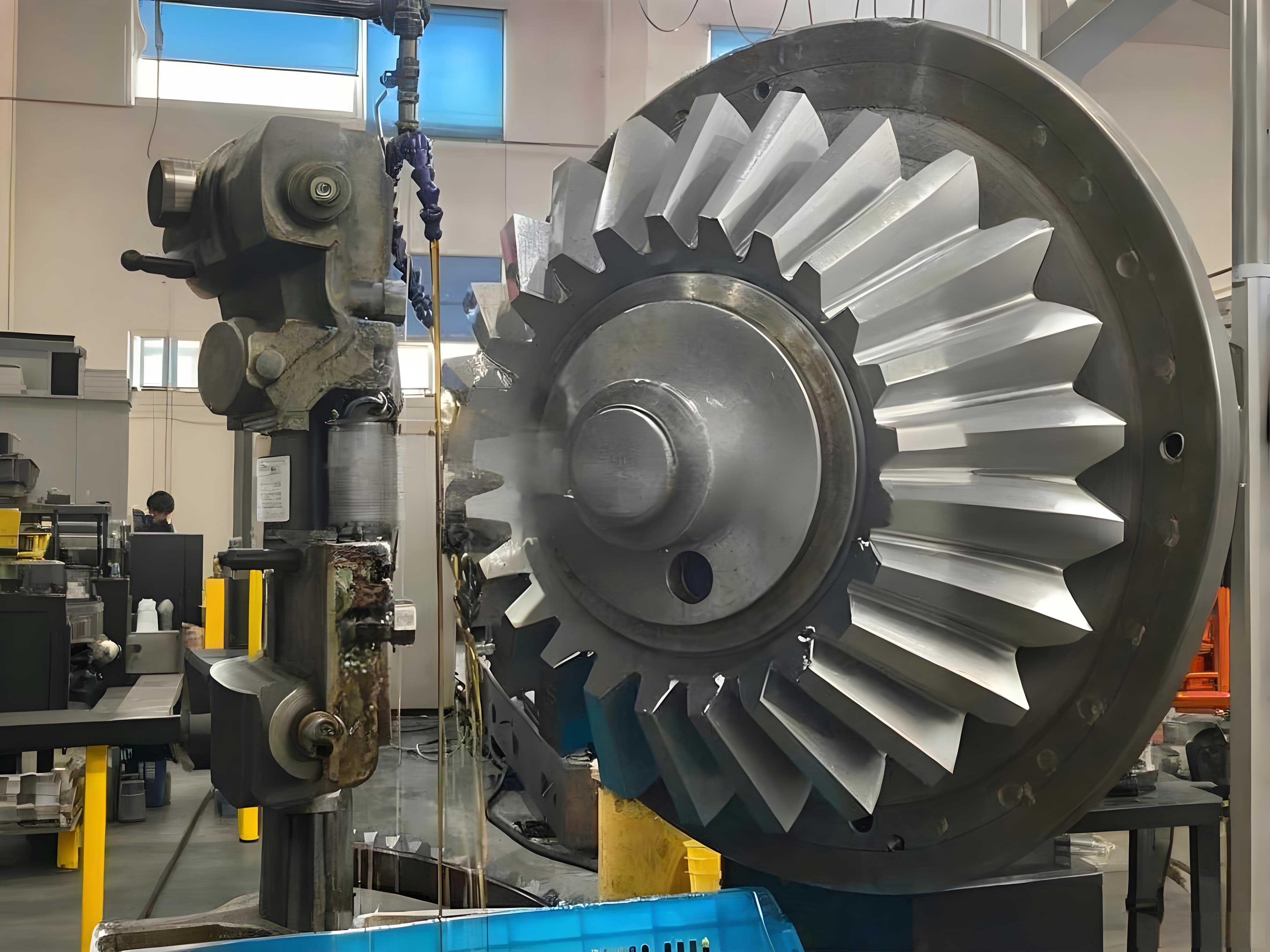
Motivation. Herringbone gear planetary systems are widely used in aerospace, marine, and heavy machinery transmissions because they combine high load capacity, compactness, and smooth transmission. In such systems, the sun gear, planet gears, and ring gear operate under repeated contact and bending loads. When a crack and pitting appear on the same tooth, the two faults interact. The crack reduces the effective load-carrying section, while pitting removes material from the tooth surface and reduces the contact width. This coupling changes the time-varying mesh stiffness, which is a primary internal excitation of the gear system. For miter gears, a comparable coupling can occur on bevel tooth flanks, and the same energy concepts can be adapted. Therefore, I treat crack-pitting coupling as a combined stiffness-reduction mechanism and examine how it propagates into the vibration response.
Scope. I focus on two meshing pairs in a planetary arrangement: the sun-planet herringbone pair and the ring-planet herringbone pair. I derive the axial compressive stiffness, bending stiffness, shear stiffness, Hertzian contact stiffness, and fillet foundation stiffness. I then introduce pitting, crack, and coupled crack-pitting damage into the effective section area and moment of inertia. I validate the analytical stiffness against a finite element model. After that, I establish a 55-degree-of-freedom bending-torsion-axial-pendulum model and solve it with a variable-step fourth-order Runge-Kutta method. I analyze time-domain waveforms, frequency spectra, phase portraits, and Poincare maps. I also evaluate crest factor, kurtosis, and sideband index as damage-sensitive indicators. Finally, I build a vibration test rig and compare measured responses with my theoretical predictions. The experience gained here can support fault diagnosis in herringbone planetary transmissions and can also inform the study of miter gears in high-load drive trains.
Geometry and slicing strategy. Because a herringbone gear can be viewed as two helical gear halves with opposite helix directions, I divide each gear into a finite number of thin slices. Each slice is treated as a narrow spur gear. The total mesh stiffness is obtained by summing the slice stiffnesses. This slicing method is efficient and avoids the high computational cost of a full three-dimensional contact model. For miter gears, the tooth form is different, but the idea of local compliance summation remains useful when miter gears are analyzed under distributed contact.
The maximum contact line length of one herringbone half is
$$ l_m=\frac{L}{\cos\beta}, $$
where \(L\) is the tooth width and \(\beta\) is the helix angle. The single-tooth contact line varies with time. I represent it as
$$ l(t)=
\begin{cases}
L_m \frac{t}{t_1}, & 0 \le t \le t_1,\\
L_m, & t_1 \le t \le t_2,\\
L_m \frac{t_3-t}{t_3-t_2}, & t_2 \le t \le t_3,
\end{cases}
$$
where \(t_1\), \(t_2\), and \(t_3\) are transition times determined by the rotational speed and tooth numbers. The multi-tooth contact line is the superposition of the active single-tooth lines. The mesh period is
$$ t_3=\frac{60}{n_1 z_1}, $$
where \(n_1\) is the driving speed and \(z_1\) is the driving tooth number. This period is used repeatedly in the vibration analysis because every time a damaged tooth enters the mesh, the stiffness disturbance repeats.
Energy components of mesh stiffness. I model each tooth as a variable-section cantilever beam. The total potential energy includes Hertzian contact energy, bending energy, shear energy, axial compressive energy, and fillet foundation energy. The corresponding stiffness components are \(k_h\), \(k_b\), \(k_s\), \(k_a\), and \(k_f\). The stored energies are
$$ U_h=\frac{F^2}{2k_h}, \quad
U_b=\int_0^d \frac{F_b^2 x^2}{2EI_x}\,dx, $$
$$ U_s=\int_0^d \frac{1.2F_b^2}{2GA_x}\,dx, \quad
U_a=\int_0^d \frac{F_a^2}{2EA_x}\,dx, $$
$$ U_f=\frac{F^2}{2k_f}. $$
Here \(E\) is Young’s modulus, \(G\) is the shear modulus, \(I_x\) is the area moment of inertia, \(A_x\) is the cross-sectional area, \(d\) is the effective distance from the root to the contact point, and \(F_b\), \(F_a\), and \(F\) are the bending, axial, and normal components of the mesh force. The Hertzian stiffness is
$$ k_h=\frac{EL}{2(1-\mu^2)}, $$
where \(\mu\) is Poisson’s ratio. For a single slice, the equivalent stiffness is
$$ k_{t,j}=\frac{1}{\frac{1}{k_{h,j}}+\frac{1}{k_{b1,j}}+\frac{1}{k_{s1,j}}+\frac{1}{k_{a1,j}}+\frac{1}{k_{f1,j}}+\frac{1}{k_{b2,j}}+\frac{1}{k_{s2,j}}+\frac{1}{k_{a2,j}}+\frac{1}{k_{f2,j}}}}, $$
and the total time-varying mesh stiffness is
$$ k_{tm}=\sum_{j=1}^{m} k_{t,j}. $$
I compute the sun-planet and ring-planet pairs separately because their tooth root geometry and pressure angle relations differ. For the sun-planet pair, I distinguish two cases: the base circle is larger than the root circle, and the base circle is smaller than the root circle. For the ring-planet pair, the root circle is generally larger than the base circle, so the expressions are adapted with the internal gear geometry. This distinction matters for crack-pitting coupling because the effective section area and moment of inertia depend on the root region and the crack path.
Stiffness formulas for the sun-planet pair. When the base circle is larger than the root circle, the bending, axial compressive, and shear stiffnesses are written as
$$ k_b=\frac{1}{\int_{a_1}^{a_2}\frac{(1+\cos a)^2}{2EL\Delta L}d a+\int_{a_2}^{a_3}\frac{(1+\cos a)^2}{2EL\Delta L}d a}, $$
$$ k_a=\frac{1}{\int_{a_1}^{a_2}\frac{\sin^2 a}{2EL\Delta L}d a+\int_{a_2}^{a_3}\frac{\sin^2 a}{2EL\Delta L}d a}, $$
$$ k_s=\frac{1}{\int_{a_1}^{a_2}\frac{1.2(1+\mu)\cos^2 a}{2EL\Delta L}d a+\int_{a_2}^{a_3}\frac{1.2(1+\mu)\cos^2 a}{2EL\Delta L}d a}. $$
When the base circle is smaller than the root circle, the integrals start from the root circle and use the corresponding section geometry. I express the effective length and half tooth thickness as
$$ d=R_b[(\cos a_1+\sin a_1)\sin a_2+\cos a_1\cos a_2]-R_f, $$
$$ h_x=R_b[\cos a_1-(\cos a_1-\sin a_1)\sin a_2]. $$
For the ring-planet pair, the angular relations include the tooth centerline angle \(\theta_0\). The bending, axial compressive, and shear stiffnesses become
$$ k_b=\frac{1}{\int_{a_f}^{a_1}\frac{3(1+\cos a)^2}{2EL\Delta L}d a}, $$
$$ k_a=\frac{1}{\int_{a_f}^{a_1}\frac{\sin^2 a}{2EL\Delta L}d a}, $$
$$ k_s=\frac{1}{\int_{a_f}^{a_1}\frac{1.2(1+\mu)\cos^2 a}{2EL\Delta L}d a}, $$
with the effective section parameters adjusted by \(\theta_0\). The fillet foundation stiffness is computed from the Muskhelishvili elastic ring formulation:
$$ \frac{1}{k_f}=\frac{\cos^2 a_m}{EL}\left[L^*\left(\frac{u_f}{S_f}\right)^2+M^*\left(\frac{u_f}{S_f}\right)+P^*\left(1+\tan^2 a_m\right)+Q^*\tan a_m\right], $$
where \(L^*\), \(M^*\), \(P^*\), and \(Q^*\) are polynomial functions of the tooth height and fillet angle. The coefficients are listed in the table below.
| Polynomial | \(A_i\) | \(B_i\) | \(C_i\) | \(D_i\) | \(E_i\) | \(F_i\) |
|---|---|---|---|---|---|---|
| \(L^*(h,\theta_f)\) | \(-5.574\times10^{-5}\) | \(-1.9986\times10^{-3}\) | \(-2.3015\times10^{-4}\) | \(4.7702\times10^{-3}\) | \(0.0271\) | \(6.8045\) |
| \(M^*(h,\theta_f)\) | \(60.111\times10^{-5}\) | \(28.100\times10^{-3}\) | \(-83.431\times10^{-4}\) | \(-9.9256\times10^{-3}\) | \(0.1624\) | \(0.9086\) |
| \(P^*(h,\theta_f)\) | \(-50.952\times10^{-5}\) | \(185.50\times10^{-3}\) | \(0.0538\times10^{-4}\) | \(53.300\times10^{-3}\) | \(0.2895\) | \(0.9236\) |
| \(Q^*(h,\theta_f)\) | \(-6.2042\times10^{-5}\) | \(9.0889\times10^{-3}\) | \(-4.0964\times10^{-4}\) | \(7.8297\times10^{-3}\) | \(-0.1472\) | \(0.6904\) |
Pitting model. I represent a single pit as a circular removal of material with depth \(h_p\) and radius \(p_d\). The pit reduces the contact width by \(\Delta L_x\), the section area by \(\Delta A_x\), and the area moment of inertia by \(\Delta I_x\). For one pit located between \(x=x_p-p_d\) and \(x=x_p+p_d\),
$$ \Delta A_x=
\begin{cases}
2h_p\sqrt{p_d^2-(x-x_p)^2}, & x\in[x_p-p_d,x_p+p_d],\\
0, & \text{otherwise},
\end{cases}
$$
$$ \Delta I_x=
\begin{cases}
\frac{1}{12}\Delta A_x\left(h_p^2+\frac{3}{4}p_d^2\right), & x\in[x_p-p_d,x_p+p_d],\\
0, & \text{otherwise},
\end{cases}
$$
$$ \Delta L_x=
\begin{cases}
2\sqrt{p_d^2-(x-x_p)^2}, & x\in[x_p-p_d,x_p+p_d],\\
0, & \text{otherwise}.
\end{cases}
$$
For multiple pits, I sum the reductions. The pitting-affected stiffnesses become
$$ k_{b-pitting}=\frac{1}{\int \frac{3(1+\cos a)^2}{E L (I_x-\Delta I_x)}d a}, $$
$$ k_{s-pitting}=\frac{1}{\int \frac{1.2(1+\mu)\cos^2 a}{E L (A_x-\Delta A_x)}d a}, $$
$$ k_{a-pitting}=\frac{1}{\int \frac{\sin^2 a}{E L (A_x-\Delta A_x)}d a}, $$
$$ k_{h-pitting}=\frac{E\left(L-\sum \Delta L_x\right)}{2(1-\mu^2)}. $$
This approach is convenient for parametric studies. The pit geometry is regular in my model, but the stiffness reduction trend is representative. In real miter gears, pits can be irregular, and the same reduction concept can be applied by integrating the local loss of area and contact width.
Crack model. I assume a straight crack initiating at the tooth root and propagating at an angle \(v\). For a cracked tooth, the effective section area and moment of inertia are
$$ A_x=
\begin{cases}
(h_x+h_c)L, & x\le d,\\
2h_xL, & x>d,
\end{cases}
$$
$$ I_x=
\begin{cases}
\frac{1}{12}(h_x+h_c)^3L, & x\le d,\\
\frac{1}{12}(2h_x)^3L, & x>d,
\end{cases}
$$
where \(h_c\) is the crack-induced height and \(d\) is the transition distance. The crack reduces the bending and shear stiffnesses. The axial compressive stiffness is less affected unless the crack is very deep. For a cracked tooth, I write
$$ k_{b-crack}=\int \frac{3(1+\cos a)^2}{E L I_x}d a, \quad
k_{s-crack}=\int \frac{1.2(1+\mu)\cos^2 a}{E L A_x}d a. $$
When the crack is shallow, the crack tip remains inside the tooth body. When the crack becomes deep, the remaining section is small, and the stiffness drops rapidly. This nonlinear reduction is important for vibration diagnosis because it creates strong periodic impulses.
Crack-pitting coupling. The coupled damage is not a simple sum of crack and pitting effects. The crack may lie inside the pitting zone, outside it, or overlap it. I define four representative coupling cases. In case 1, a light crack is combined with light pitting. In case 2, a moderate crack is combined with moderate pitting. In case 3, a severe crack fully covers the moderate pitting zone. In case 4, a moderate crack is combined with severe pitting. The coupling degree is summarized below.
| Coupling case | Crack level | Pitting level | Dominant mechanism |
|---|---|---|---|
| Case 1 | 10% | Light pitting | Crack and pitting jointly reduce stiffness |
| Case 2 | 30% | Moderate pitting | Coupled reduction in bending and shear |
| Case 3 | 60% | Moderate pitting | Crack dominates the damaged zone |
| Case 4 | 30% | Severe pitting | Pitting enlarges the contact loss |
For case 1, the bending and shear stiffnesses are
$$ k_{bcp,1}=\frac{1}{\int \frac{3(1+\cos a)^2}{E L (I_x-\Delta I_x)}d a}, \quad
k_{scp,1}=\frac{1}{\int \frac{1.2(1+\mu)\cos^2 a}{E L (A_x-\Delta A_x)}d a}. $$
For case 2, the crack and pit zones overlap, so I split the integral into a crack-only region and a coupled region:
$$ k_{bcp,2}=\frac{1}{\int_{a_2}^{a_{p1}}\frac{3(1+\cos a)^2}{E L I_x}d a+\int_{a_{p1}}^{a_{p2}}\frac{3(1+\cos a)^2}{E L (I_x-\Delta I_x)}d a}, $$
$$ k_{scp,2}=\frac{1}{\int_{a_2}^{a_{p1}}\frac{1.2(1+\mu)\cos^2 a}{E L A_x}d a+\int_{a_{p1}}^{a_{p2}}\frac{1.2(1+\mu)\cos^2 a}{E L (A_x-\Delta A_x)}d a}. $$
For case 3, the crack zone contains the entire pitting zone, so the pitting contribution is weakened. The stiffness is close to the cracked-only stiffness:
$$ k_{bcp,3}\approx k_{b-crack}, \quad k_{scp,3}\approx k_{s-crack}. $$
For case 4, severe pitting extends beyond the crack zone, so the coupled stiffness is computed with two rows of pits. The integrals include both the first and second pit rows:
$$ k_{bcp,4}=\frac{1}{\int_{a_2}^{a_{p1}}\frac{3(1+\cos a)^2}{E L I_x}d a+\int_{a_{p1}}^{a_{p2}}\frac{3(1+\cos a)^2}{E L (I_x-\Delta I_x-\Delta I_x’)}d a}, $$
$$ k_{scp,4}=\frac{1}{\int_{a_2}^{a_{p1}}\frac{1.2(1+\mu)\cos^2 a}{E L A_x}d a+\int_{a_{p1}}^{a_{p2}}\frac{1.2(1+\mu)\cos^2 a}{E L (A_x-\Delta A_x-\Delta A_x’)}d a}. $$
The prime terms denote the second pit row. This treatment captures the fact that severe pitting can remove material over a wider angular range. In miter gears, a similar coupling can occur when a root crack intersects a pitted contact zone, and the same integral split can be used.
Finite element validation. To check my analytical stiffness, I build a three-dimensional finite element model. I refine the mesh near the crack and pits, constrain the driven gear, and apply rotation to the driving gear. I extract the deformation and mesh force along the line of action. The analytical and finite element results agree well. The maximum error is below 3%. The comparison is summarized in the table below.
| Condition | Sun-planet analytical (×10⁹ N·m⁻¹) | Sun-planet FEM (×10⁹ N·m⁻¹) | Sun-planet error | Ring-planet analytical (×10⁹ N·m⁻¹) | Ring-planet FEM (×10⁹ N·m⁻¹) | Ring-planet error |
|---|---|---|---|---|---|---|
| Healthy | 1.21 | 1.23 | 1.65% | 1.43 | 1.42 | 0.70% |
| 10% crack + 3 pits | 1.14 | 1.17 | 2.63% | 1.35 | 1.37 | 1.48% |
| 30% crack + 7 pits | 0.96 | 0.97 | 1.04% | 1.18 | 1.15 | 2.61% |
| 60% crack + 7 pits | 1.03 | 1.05 | 1.94% | 1.23 | 1.25 | 1.62% |
| 30% crack + 14 pits | 0.83 | 0.85 | 2.41% | 1.03 | 1.05 | 1.94% |
The maximum reduction rates are listed below. The sun-planet pair is more sensitive to crack-pitting coupling than the ring-planet pair. This is because the sun-planet pair has a lower initial mesh stiffness and a smaller contact ratio, so a local loss of material produces a larger relative stiffness change.
| Coupling case | Sun-planet maximum reduction | Ring-planet maximum reduction |
|---|---|---|
| Case 1 | 5.78% | 5.03% |
| Case 2 | 14.03% | 13.58% |
| Case 3 | 21.48% | 20.27% |
| Case 4 | 31.40% | 27.97% |
Planetary dynamic model. I establish a 55-degree-of-freedom bending-torsion-axial-pendulum model. The sun gear, planet gears, and ring gear have translational displacements in three directions and rotational displacements about three axes. The carrier has one rotational degree of freedom. The model includes time-varying mesh stiffness, torsional stiffness, mesh damping, backlash, comprehensive mesh error, and the cutter relief groove. The relief groove is represented as a torsional connection between the left and right helical halves of each herringbone gear. This is important because the two halves do not behave as a single rigid body when the groove is flexible.
The relative displacement of the sun-planet pair along the line of action is
$$ \delta_{spi}^{g}=
x_s^g\sin\psi_{spi}+y_s^g\cos\psi_{spi}
-r_s\theta_s^g
-x_{pi}^g\sin\alpha_E
-y_{pi}^g\cos\alpha_E
+r_{pi}\theta_{pi}^g
+(-1)^{g}(z_s^g-z_{pi}^g)\sin\beta
-e_{spi}^g(t), $$
where \(g=L,R\) denotes the left and right halves, \(\psi_{spi}\) is the mesh line angle, \(\alpha_E\) is the transverse pressure angle, \(r_s\) and \(r_{pi}\) are base radii, and \(e_{spi}^g(t)\) is the comprehensive mesh error. For the ring-planet pair,
$$ \delta_{rpi}^{g}=
x_r^g\sin\psi_{rpi}+y_r^g\cos\psi_{rpi}
-x_{pi}^g\sin\alpha_I
-y_{pi}^g\cos\alpha_I
+r_{pi}\theta_{pi}^g
+(-1)^{g}(z_r^g-z_{pi}^g)\sin\beta
-e_{rpi}^g(t). $$
The planet-carrier relative displacements are
$$ \delta_{cpi x}^{g}=x_{pi}^g-x_c\cos\varphi_i-y_c\sin\varphi_i, $$
$$ \delta_{cpi y}^{g}=y_{pi}^g-x_c\sin\varphi_i+y_c\cos\varphi_i, $$
$$ \delta_{cpi z}^{g}=z_{pi}^g-z_c. $$
I write the equations of motion in matrix form as
$$ \mathbf{M}\ddot{\mathbf{X}}+\mathbf{C}\dot{\mathbf{X}}+\mathbf{K}\mathbf{X}=\mathbf{F}, $$
where \(\mathbf{M}\) is the mass matrix, \(\mathbf{C}\) is the damping matrix, \(\mathbf{K}\) is the stiffness matrix, \(\mathbf{X}\) is the displacement vector, and \(\mathbf{F}\) is the excitation vector. The stiffness matrix contains the time-varying mesh stiffness, the support stiffness, the torsional stiffness, and the relief-groove stiffness. The damping matrix contains the mesh damping and the support damping. The excitation vector contains the comprehensive mesh error, the static transmission error, and the external torque.
Internal excitations. I compute the comprehensive mesh error from manufacturing error, installation error, and eccentricity. For the sun-planet pair,
$$ e_{spi}^g=e_{Ms}^g+e_{Mpi}^g+e_{Mc}^g+e_{Ipi}^g+e_{Is}^g. $$
For the ring-planet pair,
$$ e_{rpi}^g=e_{Mr}^g+e_{Mpi}^g+e_{Is}^g+e_{Ipi}^g. $$
The mesh damping is
$$ c_{spi}=2\zeta_{spi}\sqrt{\frac{k_{spi}}{1/m_s+1/m_p}}, \quad
c_{rpi}=2\zeta_{rpi}\sqrt{\frac{k_{rpi}}{1/m_r+1/m_p}}. $$
The backlash function is
$$ f(x)=
\begin{cases}
x-b, & x>b,\\
0, & -b\le x\le b,\\
x+b, & x<-b.
\end{cases}
$$
These nonlinear elements are included in the numerical integration. They create rich dynamic behavior, especially when crack-pitting coupling reduces the mesh stiffness and increases the dynamic transmission error.
Characteristic frequencies. For a sun-input, ring-fixed, carrier-output planetary system, the transmission ratio is
$$ i=1+\frac{z_r}{z_s}. $$
The sun rotation frequency is
$$ f_s=\frac{n}{60}. $$
The carrier frequency is
$$ f_c=\frac{f_s}{i}. $$
The mesh frequency is
$$ f_m=(f_s-f_c)z_s=(f_s-f_c)z_p=(f_c-f_r)z_r. $$
The crack-pitting characteristic frequency is
$$ f_g=\frac{f_m}{z_s N}, $$
where \(N\) is the number of planets. In my case, \(f_m=480\) Hz and \(f_g=80\) Hz. The sun rotation period is 0.03 s, and the coupled fault period is 0.0125 s. These values match the periodic impact spacing in the simulated and measured signals.
Numerical solution. I solve the nonlinear differential equations with a variable-step fourth-order Runge-Kutta method. The update formula is
$$ y_{n+1}=y_n+\frac{h}{6}(k_1+2k_2+2k_3+2k_4), $$
$$ k_1=f(t_n,y_n), \quad
k_2=f\left(t_n+\frac{h}{2},y_n+\frac{h}{2}k_1\right), $$
$$ k_3=f\left(t_n+\frac{h}{2},y_n+\frac{h}{2}k_2\right), \quad
k_4=f(t_n+h,y_n+hk_3). $$
I set the sun speed to 2000 r/min and the input torque to 400 N·m. I fix the ring gear and use the sun as input and the carrier as output. The time step is chosen to resolve the mesh frequency and the crack-pitting sidebands. I discard the first part of the response to remove transient effects, and then I analyze the steady-state response.
Vibration response without damage. When the sun gear is healthy, the time-domain displacement is smooth and periodic. The displacement range is about \(-7.21\) μm to \(-10.77\) μm in the x-direction. The frequency spectrum is dominated by the mesh frequency \(f_m\), the second harmonic \(2f_m\), and the third harmonic \(3f_m\). The amplitudes are approximately \(9.7\times10^{-2}\) μm, \(5.9\times10^{-2}\) μm, and \(0.84\times10^{-2}\) μm. The phase portrait is a closed and regular ring, and the Poincare map consists of a small number of concentrated points. This indicates periodic motion and a stable operating condition.
Vibration response with a single crack. When the sun gear has a 30% crack, the time-domain signal shows periodic impulses. The displacement range expands to about \(-6.73\) μm to \(-11.38\) μm. Because there are three planets, the cracked tooth meshes with each planet once per sun revolution. Therefore, three impulses appear in one sun rotation period. The frequency spectrum contains the mesh frequency and its harmonics, and sidebands appear around them. The crack-pitting characteristic frequency \(f_g=80\) Hz is also visible. The phase portrait becomes a set of non-overlapping rings, and the Poincare map contains more discrete points. The system remains periodic but the motion is more complex than the healthy case.
Vibration response with single pitting. When the sun gear has six pits, the time-domain signal also shows periodic impulses, but the impulse amplitude is smaller than in the crack case. The displacement range is about \(-6.91\) μm to \(-11.25\) μm. The frequency spectrum shows sidebands around the mesh frequency, but the sideband amplitude is lower than in the crack case. This is because pitting mainly reduces the contact width, while a crack reduces the load-carrying section and changes the bending flexibility more strongly. The phase portrait is more scattered than the healthy case but less scattered than the crack case.
Vibration response with crack-pitting coupling. For coupling case 2, the displacement range is about \(-6.34\) μm to \(-11.62\) μm. The impulse amplitude is the largest among the three single-fault and coupled cases. The frequency spectrum shows strong sidebands around \(f_m\) and its harmonics. The sideband spacing is \(f_g\), and the sideband amplitude increases with coupling severity. The phase portrait becomes a multi-ring structure, and the Poincare map becomes more dispersed. These features indicate that crack-pitting coupling produces a stronger internal excitation than either crack or pitting alone.
For coupling case 3, the crack zone fully covers the pitting zone. The time-domain response is close to the response of the 60% crack case. The displacement range is about \(-5.72\) μm to \(-12.38\) μm. The frequency spectrum is also similar to the crack-dominated case. This confirms that when the crack affects the entire damaged region, the pitting contribution becomes secondary. For miter gears, a similar transition can occur when a root crack grows through a pitted region and the crack becomes the controlling compliance source.
For coupling case 4, the pitting level is severe while the crack remains moderate. The displacement range is about \(-5.93\) μm to \(-12.12\) μm. The sidebands and the characteristic frequency amplitude are larger than in case 2. This shows that severe pitting can significantly enlarge the coupled fault signature even when the crack does not fully dominate. The dynamic response therefore depends on both the crack size and the pitting severity, and neither parameter alone is sufficient to describe the fault.
Signal indicators. I use crest factor, kurtosis, and sideband index to quantify the vibration response. The root mean square is
$$ RMS=\sqrt{\frac{1}{N}\sum_{i=1}^{N}x(i)^2}. $$
The crest factor is
$$ CF=\frac{\max |x(i)-\bar{x}|}{RMS}. $$
The kurtosis is
$$ K=\frac{\frac{1}{N}\sum_{i=1}^{N}(x(i)-\bar{x})^4}{\left[\frac{1}{N}\sum_{i=1}^{N}(x(i)-\bar{x})^2\right]^2}. $$
The sideband index is
$$ SI=\frac{1}{M}\sum_{k=1}^{M}|X(k)|, $$
where \(X(k)\) are the amplitudes in the first-order sideband. The percentage increment is
$$ \Delta\delta=\frac{\delta(i)-\delta}{\delta}\times100\%. $$
The indicator results are summarized below. Kurtosis and sideband index are more sensitive to crack-pitting coupling than crest factor. As the coupling severity increases, all three indicators increase, but kurtosis shows the largest relative change. This makes kurtosis a good candidate for detecting crack-pitting coupling in herringbone planetary systems. The sideband index is also useful because it directly reflects the frequency-domain modulation caused by the fault.
| Indicator | Light pitting minimum | Light pitting maximum | Moderate pitting minimum | Moderate pitting maximum | Severe pitting minimum | Severe pitting maximum |
|---|---|---|---|---|---|---|
| Crest factor increment | 1.05% | 30.33% | 3.32% | 78.88% | 5.21% | 83.26% |
| Kurtosis increment | 0.52% | 104.15% | 8.78% | 124.04% | 30.81% | 133.05% |
| Sideband index | 1.03 | 2.02 | 1.17 | 2.18 | 1.32 | 2.26 |
Experimental validation. I build a vibration test rig for the herringbone planetary system. The rig includes a drive motor, a herringbone planetary gearbox, an acceleration sensor, a torque sensor, a magnetic powder brake, and a multi-channel data acquisition system. I install the acceleration sensor on the gearbox housing near the input bearing. I measure the acceleration signal and then integrate it twice to obtain the displacement signal. I use a sampling frequency of 51200 Hz and a sampling time of 20 s. The input speed is 2000 r/min, the mesh frequency is 480 Hz, and the crack-pitting characteristic frequency is 80 Hz.
I manufacture the damaged gears by wire-cut electrical discharge machining. I first cut a helical gear into two halves, then machine a left-hand and a right-hand half, and finally assemble them into a herringbone gear. I introduce a 45-degree crack and circular pits with a diameter of 1 mm. The gear accuracy is grade 6. This manufacturing route allows me to control the crack angle, crack length, pit diameter, and pit distribution. It also allows me to compare healthy, cracked, pitted, and coupled gears under the same operating conditions.
The measured healthy response is smooth and periodic. The displacement range is about \(-4.74\) μm to \(4.98\) μm. The frequency spectrum is dominated by the mesh frequency, and the sidebands are weak. When the sun gear contains six pits and a 30% crack, the time-domain signal shows clear periodic impulses. The impulse period is 0.0125 s, which matches the theoretical crack-pitting period. The frequency spectrum shows sidebands around the mesh frequency and its harmonics, and the characteristic frequency \(f_g=80\) Hz is visible. When the sun gear contains twelve pits and a 30% crack, the sidebands become stronger, and the impulse amplitude increases. These experimental trends agree with my theoretical results.
The comparison between theory and experiment is shown below. The absolute amplitudes differ because the theoretical model does not include the full gearbox housing, shafts, bearings, and foundation. However, the trend and the characteristic frequencies are consistent. This validates the dynamic model and the crack-pitting stiffness formulation. For miter gears, a similar experimental strategy can be used by introducing controlled pitting and root cracks on bevel teeth and measuring the resulting vibration signature.
| Condition | Theoretical maximum displacement (μm) | Experimental maximum displacement (μm) | Main observed frequency |
|---|---|---|---|
| Healthy | 10.77 | 4.98 | \(f_m\) |
| 30% crack + 6 pits | 11.62 | 8.20 | \(f_m,\ f_g,\ f_m\pm f_g\) |
| 30% crack + 12 pits | 12.12 | 10.40 | \(f_m,\ f_g,\ f_m\pm f_g\) |
Discussion. The crack-pitting coupling changes the mesh stiffness in two ways. First, the crack reduces the bending and shear stiffness by decreasing the effective section area and moment of inertia. Second, the pits reduce the contact width and the Hertzian stiffness. When the two faults overlap, the stiffness reduction is larger than the reduction from either fault alone. When the crack fully covers the pitting zone, the crack becomes the dominant factor, and the stiffness curve approaches the cracked-only curve. When the pitting extends beyond the crack, the contact loss becomes dominant, and the sideband energy increases. These transitions are important for fault diagnosis because they change the relationship between damage size and vibration amplitude.
The planetary system adds another layer of complexity. Because there are three planets, the damaged sun tooth meshes with each planet once per sun revolution. This produces three impulses per revolution and creates modulation sidebands around the mesh frequency. The ring-planet pair also contributes to the response, but its sensitivity is lower than that of the sun-planet pair. The sun-planet pair is therefore the best location for early detection of crack-pitting coupling. In miter gears used in intersecting-axis drives, the same principle applies: the pair with the smaller contact ratio and lower initial stiffness will usually show the strongest relative stiffness change.
The relief groove is also important. I model the groove as a torsional spring between the left and right halves. If the groove is stiff, the two halves act nearly as one gear. If the groove is flexible, the two halves can oscillate relative to each other, and this adds additional vibration modes. The crack-pitting fault can excite these modes, especially when the fault is on one half of the herringbone tooth. This is a feature that distinguishes herringbone gears from simple spur or helical gears. For miter gears, the equivalent feature is the compliance of the hub and the shaft connection, which can also couple with tooth faults.
Design and monitoring implications. My results suggest several practical guidelines. First, crack-pitting coupling should be treated as a distinct fault class, not as a simple superposition of crack and pitting. Second, the sideband index and kurtosis are more sensitive than the crest factor, so they should be used together for condition monitoring. Third, the sun-planet mesh should be monitored with priority because it is more sensitive to coupling. Fourth, the characteristic frequency \(f_g\) and the sidebands \(f_m\pm f_g\) should be included in diagnostic algorithms. Fifth, the transition from pitting-dominant to crack-dominant behavior can be detected by comparing the sideband amplitude with the mesh stiffness reduction. These guidelines are also relevant to miter gears and other high-load gear types.
Limitations and future work. I use regular pit shapes and a straight crack path to make the model tractable. In reality, pits are irregular, and cracks propagate along curved paths. I also neglect tooth friction and thermal effects. These simplifications affect the absolute amplitude but not the main trends. In future work I will extend the model to curved crack paths, irregular pit shapes, and mixed lubrication. I will also include the gearbox housing and bearings in the dynamic model and use a direct gear vibration measurement method to reduce the influence of housing flexibility. These improvements will make the prediction more accurate for both herringbone planetary systems and miter gears.
Conclusions. I have developed an analytical and numerical framework for the time-varying mesh stiffness and vibration of a herringbone planetary system with crack-pitting coupling. The main findings are as follows. The crack-pitting coupled stiffness is lower than the stiffness of either single fault. When the crack zone covers the pitting zone, the crack dominates the stiffness reduction. When the pitting zone extends beyond the crack, the contact loss dominates the sideband response. The sun-planet pair is more sensitive to crack-pitting coupling than the ring-planet pair. The 55-degree-of-freedom dynamic model reproduces the periodic impulses, the characteristic frequency \(f_g\), and the sidebands around the mesh frequency. The experimental results confirm the theoretical trends. Kurtosis and sideband index are the most sensitive indicators. The results provide a basis for fault diagnosis and reliability improvement in herringbone planetary transmissions, and they can also guide the study of miter gears under combined surface and root damage.
| Parameter | Sun | Planet | Ring | Carrier |
|---|---|---|---|---|
| Module (mm) | 2 | 2 | 2 | — |
| Tooth number | 18 | 27 | 72 | — |
| Face width (mm) | 60 | 60 | 70 | — |
| Normal pressure angle (deg) | 20 | 20 | 20 | — |
| Helix angle (deg) | 16 | 16 | 16 | — |
| Mass (kg) | 1.49 | 2.86 | 3.24 | 1.98 |
| Moment of inertia (kg·m²) | 0.028 | 0.042 | 0.116 | 0.15 |
| Poisson’s ratio | 0.3 | 0.3 | 0.3 | 0.3 |
| Young’s modulus (GPa) | 207 | 207 | 207 | 207 |
In summary, my study connects local crack-pitting damage to global vibration in a herringbone planetary system. The combination of energy-based stiffness, finite element validation, nonlinear dynamic simulation, and experimental testing provides a consistent picture of the fault behavior. The same logic can be transferred to miter gears, where surface pitting and root cracking can also coexist and interact. I believe the proposed framework can support the design of more reliable gear transmissions and the development of more sensitive condition-monitoring methods.