
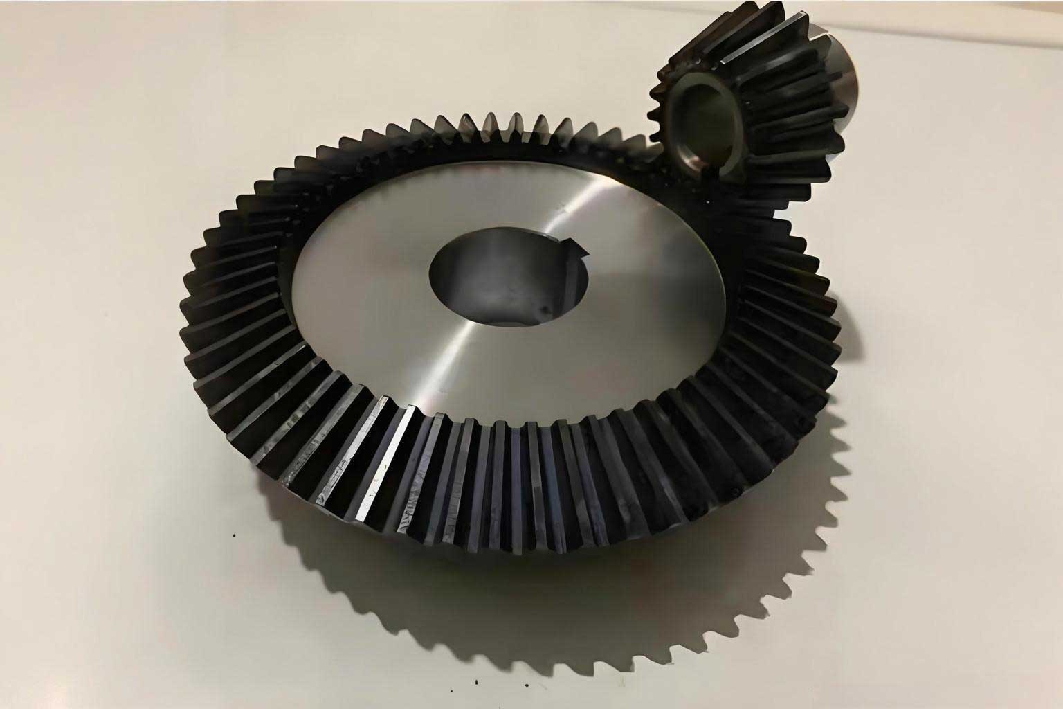
In my research, I examined the form grinding process of miter gears, using a herringbone gear as the main representative case for high-load aerospace transmission systems. Miter gears are widely associated with compact motion transfer, but the broader class of miter gears includes several gear forms that must be finished by grinding when high surface integrity and geometric accuracy are required. I focused on how miter gears can be manufactured with larger grinding wheels, lower grinding force, better surface quality, and stronger collaboration between design and manufacturing. The central idea in my work is that miter gears with opposite helical directions and a central clearance groove have unused space around the tooth slots and the clearance groove. If this space is used correctly, a grinding wheel can borrow space from an opposite tooth slot, a clearance groove, or an opposite adjacent tooth slot. I call this method the wheel–miter gear borrowing grinding method.
I organized the study into three connected parts. First, I optimized the grinding process and defined a quantitative borrowing coefficient for miter gears. Second, I built maximum wheel diameter models for clearance-groove borrowing and tooth-slot borrowing, corrected them for wheel thickness, backlash, and over-center grinding, and validated them by simulation and machining. Third, I developed a grinding force prediction model for miter gears by considering abrasive grain morphology, double-grain shadowing, sliding, ploughing, and chip formation. I then conducted grinding experiments and embedded the results into a process software tool for design–manufacturing collaboration.
Process Requirements and the Need for Wheel Diameter Expansion
I began with the practical problem that larger grinding wheels generally improve grinding efficiency, wheel life, heat dissipation, and profile consistency. In miter gears, however, the central clearance groove and the limited internal space often restrict wheel diameter. A larger wheel means a larger contact area, fewer wheel changes, and a more stable dressing allowance. For miter gears used in aerospace systems, this advantage is especially important because the parts are often small, light, and highly loaded. The contradiction is clear: miter gears need compact designs and high power-to-weight ratios, while manufacturing needs larger wheels for quality and productivity.
I found that the traditional approach is to increase the clearance groove width so that a larger wheel can enter the grinding zone. However, increasing the clearance groove width raises the axial size and mass of miter gears. In some aerospace applications, reducing the clearance groove width by only 1 mm can save a considerable amount of mass at the system level. Therefore, I treated the wheel diameter expansion problem and the clearance groove reduction problem as two sides of the same optimization problem. My objective was to use the existing empty space of miter gears rather than simply enlarging the clearance groove.
In the conventional grinding setup, the motions between the wheel and the miter gear are already standardized. The gear rotates, the wheel rotates, and the machine provides translation and swivel motions. I observed that the standard setup does not automatically use the opposite tooth slot or the opposite adjacent tooth slot. This unused spatial relationship is the key to my borrowing method. I therefore analyzed the spatial position of the wheel relative to the miter gear and divided the borrowing behavior into three forms: borrowing the opposite tooth slot, borrowing the clearance groove, and borrowing the opposite adjacent tooth slot. These three forms are not merely geometrical descriptions; I quantified them with a borrowing coefficient and then used that coefficient to judge feasibility.
Borrowing Grinding Method for Miter Gears
The miter gear in my study has two opposite helical sides and a central clearance groove. If the helix angle, normal module, and tooth number are chosen appropriately, the wheel can pass through the clearance groove and enter a region that belongs geometrically to the opposite tooth slot. The wheel does not cut the opposite flank because the contact condition is controlled by the relative position of the wheel profile and the gear profile. I described this as a borrowing action because the wheel uses a spatial region that is not occupied by the current tooth slot during a part of the grinding cycle.
To quantify the borrowing condition, I considered the pitch cylinder and the arc length between tooth slots. I defined the borrowing coefficient \(K\) by relating the normal module \(m_n\), the helix angle \(\beta\), and the clearance groove width \(L\):
$$ \frac{\pi m_n}{\sin\beta}=L K $$
Equivalently,
$$ K=\frac{\pi m_n}{L\sin\beta} $$
I interpreted \(K\) as a dimensionless indicator of how far the wheel can borrow from the opposite side of the miter gear. The value of \(K\) is affected by the tooth number \(Z\), the pitch radius \(R\), the helix angle \(\beta\), the normal module \(m_n\), and the clearance groove width \(L\). I also introduced a profile deviation function \(H(K)\) to describe how the wheel profile moves away from the gear profile as the borrowing coefficient changes:
$$ H(K)=\frac{\pi m_n\left(K\sin\beta-Z\beta\right)}{\sin\beta\cos\beta} $$
Although this expression is derived from an idealized geometry, it helped me establish the meaningful range of \(K\). When \(K\) becomes too large, the wheel profile and the miter gear profile diverge so much that interference is no longer possible. In my calculations, values beyond 3 were not useful for the borrowing problem because the profiles separated over the relevant tooth span. Therefore, I limited the practical range to \(0<k<3\).
I further studied the application range of the borrowing coefficient. The feasible borrowing region lies between two boundary values \(K_a\) and \(K_b\), which correspond to intersections of the involute profile with the pitch circle. I included backlash \(J_t\), tooth thickness \(S_m\), pitch arc length \(S_p\), and a safety margin \(\delta\). The boundary values can be written as:
$$ K_a=0.75-\frac{J_t}{S_p}+\delta $$
$$ K_b=1.25+\frac{J_t}{S_p}-\delta $$
For an unmodified miter gear in the design stage, I found that the tooth-slot borrowing range is most meaningful when \(K\) is near 1. Values near 0.75 and 1.25 define the boundaries. Values below 0.25 correspond to a very small helix angle and are not attractive for miter gears. Values above 1.75 usually mean that the wheel and the miter gear are already separated. Table 1 summarizes the numerical distribution and the physical meaning that I assigned to the borrowing coefficient.
| Range of \(K\) | Wheel condition | Borrowing assessment |
|---|---|---|
| \([0,0.25)\) | Borrows opposite tooth slot | Rare, helix angle is too small |
| \([0.25,0.75)\) | Interferes with opposite flank | Not suitable for borrowing |
| \([0.75,1.25)\) | Borrows opposite adjacent tooth slot | Common for \(\beta\approx15^\circ-35^\circ\) |
| \([1.25,1.75)\) | Interferes with opposite adjacent flank | Not suitable for borrowing |
| \([1.75,+\infty)\) | No interference | Rare, helix angle is too large |
Table 1 shows that the most useful interval for miter gears is \([0.75,1.25)\). In this interval, the wheel can borrow the opposite adjacent tooth slot while still maintaining a stable contact condition. I then used this result to support design–manufacturing collaboration. In the design stage, engineers can choose \(L\), \(\beta\), and \(m_n\) so that \(K\) falls inside the useful interval. In the manufacturing stage, operators can use the same coefficient to judge whether a miter gear can be ground by borrowing. This avoids blind trial cuts and reduces the risk of damaging the tooth surface.
Design and Manufacturing Collaboration for Miter Gears
I treated the borrowing coefficient as a bridge between design and manufacturing. Traditional serial development often separates the design office from the shop floor. Designers may specify a compact clearance groove without knowing whether the available wheel can enter the grinding zone. Operators may struggle with a wheel that is too small and may compensate by increasing processing time. For miter gears, this problem is severe because the clearance groove is small and the wheel diameter has a strong influence on efficiency.
Using the relation between \(K\), \(L\), \(\beta\), and \(m_n\), I created a mapping surface for the ideal borrowing condition \(K=1\). On this surface, every combination of \(L\), \(\beta\), and \(m_n\) is in a balanced borrowing state. I used this surface to help designers select parameters for miter gears that are both compact and manufacturable. If the maximum wheel diameter for non-borrowing and borrowing conditions is known, the clearance groove width can be reduced while maintaining a suitable wheel size. This directly supports mass reduction and compact design. Table 2 gives an example of how the borrowing coefficient can guide parameter selection for miter gears.
| \(m_n\) (mm) | \(\beta\) (deg) | \(L\) for \(K=1\) (mm) | Design implication |
|---|---|---|---|
| 1.5 | 25 | 11.15 | Compact miter gear, moderate borrowing |
| 1.7 | 27 | 11.77 | Good balance for small miter gears |
| 2.0 | 30 | 12.57 | Higher load capacity, larger groove |
| 2.5 | 32 | 14.82 | Strong borrowing potential |
| 3.0 | 35 | 15.69 | Large module, robust wheel access |
I concluded that the borrowing method is not only a machining trick. It is also a design principle for miter gears. The same relation can be used to reduce the clearance groove, increase the wheel diameter, and improve the power-to-weight ratio. This is why I later converted the mathematical model into a software tool. The software allows designers and operators to evaluate miter gears with a common numerical language.
Maximum Wheel Diameter Modeling for Clearance-Groove Borrowing
I first modeled the simpler case in which the wheel borrows only the clearance groove. The wheel diameter \(D\) is solved from the triangle formed by the wheel center, the gear center, and the contact point on the tooth slot. I used the pitch radius \(R\), the tip radius \(R_u\), the clearance groove width \(L\), and the helix angle \(\beta\). The intermediate lengths are:
$$ ab=L $$
$$ ac=\frac{L}{\cos\beta} $$
$$ ao=\sqrt{R^2+ab^2} $$
$$ co=\sqrt{R^2+L^2} $$
Then the angle between \(ac\) and \(ao\) is found by the cosine rule:
$$ \cos(\angle cao)=\frac{ac^2+ao^2-co^2}{2ac\cdot ao} $$
The contact length \(cd\) is obtained from the triangle \(acd\):
$$ cd=\sqrt{ac^2+ad^2-2ac\cdot ad\cos(\angle cao)} $$
where
$$ ad=ao-R_u $$
I also introduced an auxiliary angle related to the tooth spacing. If \(gd\) is the lateral projection of the contact geometry, then
$$ gd=ad\cos(\angle gda),\qquad \angle gda=\frac{2\pi}{Z} $$
and
$$ \sin(\angle gcd)=\frac{gd}{cd} $$
The final wheel diameter \(D\) for clearance-groove borrowing is obtained from the triangle whose vertices include the wheel center. I write it in compact form as:
$$ D=\frac{cd^2+h^2+2cd\,h\cos(\angle dco+h)}{2\left(cd\,\cos(\angle dco+h)+h\right)} $$
Here \(h\) represents the vertical offset between the wheel center and the reference line. This expression gives the largest wheel diameter that can pass through the clearance groove without interfering with the opposite flank. It is the basis for the more complex tooth-slot borrowing model.
Maximum Wheel Diameter Modeling for Tooth-Slot Borrowing
For tooth-slot borrowing, the wheel must pass the opposite adjacent tooth slot and then contact the desired flank. This case is more difficult because the wheel center is not aligned with the clearance groove. I used a curved surface triangle on the pitch cylinder to account for the helical twist. I defined \(w\) as the face width and \(e\) as the projection related to the opposite tooth slot. The length of the helical twist is:
$$ ee’ = \frac{w}{\cos\beta}\sqrt{\tan^2\beta-1} $$
and the corresponding projected length is:
$$ en = \frac{2\sin\beta}{R}w $$
I then computed the depth \(df’\) using the law of sines in the curved triangle:
$$ df’=\frac{ne’\sin(\angle ne’e)}{\cos(\angle ne’e-\beta)} $$
The auxiliary relations are:
$$ \angle ne’e=\arcsin\left(\frac{w}{e’n}\right) $$
$$ e’d=ee’+ed $$
The radial drop caused by the helical twist is:
$$ \Delta f=\sqrt{df’^2+R_u^2}-R_u\sin\beta $$
The small angle between the clearance-groove direction and the tooth-slot borrowing direction is:
$$ \angle fcf’=\tan^{-1}\left(\frac{\Delta f}{df’+cd}\right) $$
The length \(ED\) represents the extra space needed for over-center grinding. I expressed it as:
$$ ED=C_{cn}\sin\beta $$
and the associated lateral length as:
$$ EL=C_{cn}\sin\beta\cos\beta $$
where \(C_{cn}\) is the half-width of the tooth slot on the tip cylinder:
$$ C_{cn}=R_u\left(\frac{\pi}{Z}-\frac{S_u}{2R_u}\right) $$
The tip arc tooth thickness \(S_u\) is:
$$ S_u=S_m\frac{R_u}{R_m}+2R_u\left(\operatorname{inv}\alpha_u-\operatorname{inv}\alpha_m\right) $$
and the reference arc thickness and pitch radius are:
$$ S_m=\frac{\pi m_n}{2\cos\beta},\qquad R_m=\frac{m_n Z}{2\cos\beta} $$
The involute functions are:
$$ \operatorname{inv}\alpha_m=\tan\alpha_m-\alpha_m $$
$$ \operatorname{inv}\alpha_u=\tan\alpha_u-\alpha_u $$
After correction for wheel thickness and backlash, I replaced the straight length \(f’c\) by a corrected value \(FC\):
$$ FC=\frac{U\,df’+V\,cd}{\cos(\angle fcf’)} $$
where \(U(K)\) and \(V(K)\) are correction functions obtained from contact simulation. I constructed them as:
$$ U(K)=\cos(2\pi K) $$
$$ V(K)=1+\frac{K-1}{\sin\beta}L $$
These functions are not arbitrary; they reflect the lateral movement and local contact of the wheel as \(K\) changes. I then obtained the corrected maximum wheel diameter for tooth-slot borrowing:
$$ D_{Max}=\frac{FC^2+h^2+2FC\,h\cos(\angle fco+h)}{2\left(FC\,\cos(\angle fco+h)+h\right)} $$
For over-center grinding compensation, I updated the expressions to include \(ED\). The final corrected forms are:
$$ D=\frac{cd^2+ED^2+h^2+2cd\,ED\cos(\angle dco+h)}{2\left(cd\,\cos(\angle dco+h)+h\right)} $$
$$ D_{Max}=\frac{FC^2+ED^2+h^2+2FC\,ED\cos(\angle fco+h)}{2\left(FC\,\cos(\angle fco+h)+h\right)} $$
I also updated the minimum clearance groove width when over-center grinding is required:
$$ L_{\min}=L+ED $$
These corrections are important because the wheel thickness and the tooth-side clearance change the actual contact condition. Without these corrections, the model tends to overestimate the available space. I validated all key variables by contact simulation and actual machining.
Simulation and Machining Validation for Miter Gears
I used solid contact simulation to verify the intermediate variables that are difficult to measure directly. I studied twelve typical miter gear models with different modules, tooth numbers, face widths, and clearance grooves. Table 3 lists the structural parameters used in the simulation.
| Model | \(m_n\) (mm) | \(\beta\) (deg) | \(\alpha\) (deg) | \(Z\) | \(W\) (mm) | \(L\) (mm) | \(\phi_u\) (mm) | \(\phi_d\) (mm) |
|---|---|---|---|---|---|---|---|---|
| 1 | 3.81 | 30 | 22.5 | 23 | 41 | 19 | 110.41 | 118.5 |
| 2 | 3.81 | 30 | 22.5 | 88 | 41 | 19 | 517.33 | 525.3 |
| 3 | 2.93 | 30 | 22.5 | 20 | 42 | 19 | 81.21 | 78.15 |
| 4 | 2.93 | 30 | 22.5 | 116 | 42 | 19 | 302.18 | 218.5 |
| 5 | 3.12 | 30 | 22.5 | 30 | 28 | 19 | 100.16 | 90.81 |
| 6 | 3.12 | 30 | 22.5 | 105 | 28 | 19 | 360.12 | 308.2 |
| 7 | 3.17 | 30 | 22.5 | 31 | 51 | 19 | 150.10 | 111.4 |
| 8 | 3.17 | 30 | 22.5 | 90 | 51 | 19 | 636.22 | 617.2 |
| 9 | 6.0 | 30 | 22.5 | 24 | 38 | 19 | 155.1 | 117.8 |
| 10 | 5.0 | 30 | 22.5 | 21 | 38 | 19 | 141.78 | 113.1 |
| 11 | 3.11 | 30 | 22.5 | 26 | 13.6 | 14 | 67.25 | 62.98 |
| 12 | 2.11 | 30 | 22.5 | 38 | 13.6 | 14 | 88.55 | 83.33 |
I used the over-center grinding distance \(ED\) as one of the most sensitive intermediate variables. Table 4 compares the model value \(ED\) with the simulated value \(ED’\). The average relative error was 4.45%, which I considered acceptable for an intermediate geometric variable.
| Model | \(ED\) (mm) | \(ED’\) (mm) | Error (%) |
|---|---|---|---|
| 1 | 3.183 | 3.281 | 2.987 |
| 2 | 2.771 | 3.000 | 7.633 |
| 3 | 2.181 | 2.168 | 0.600 |
| 4 | 1.711 | 1.911 | 10.466 |
| 5 | 1.987 | 2.073 | 4.149 |
| 6 | 1.862 | 1.954 | 4.708 |
| 7 | 3.088 | 3.221 | 4.129 |
| 8 | 2.872 | 3.012 | 4.648 |
| 9 | 3.005 | 3.040 | 1.151 |
| 10 | 2.911 | 3.031 | 3.959 |
| 11 | 1.137 | 1.174 | 3.152 |
| 12 | 1.077 | 1.143 | 5.774 |
I then compared the model-calculated wheel diameters with the contact simulation results. Table 5 shows the borrowing coefficient, the borrowing decision, the clearance-groove wheel diameter \(D\), the tooth-slot wheel diameter \(D_{Max}\), and their simulated counterparts.
| Model | \(K\) | Borrowing | \(D\) (mm) | \(D’\) (mm) | Error (%) | \(D_{Max}\) (mm) | \(D’_{Max}\) (mm) | Error (%) |
|---|---|---|---|---|---|---|---|---|
| 1 | 0.721 | Yes | 48.745 | 49.195 | 0.915 | 64.334 | 68.000 | 5.391 |
| 2 | 0.721 | Yes | 48.938 | 48.186 | 1.573 | 59.037 | 63.000 | 6.290 |
| 3 | 1.166 | No | 80.705 | 86.609 | 6.817 | — | — | — |
| 4 | 1.166 | No | 75.974 | 75.051 | 0.132 | — | — | — |
| 5 | 1.158 | Yes | 90.617 | 93.961 | 3.559 | 118.422 | 128.159 | 7.598 |
| 6 | 1.158 | Yes | 82.469 | 82.514 | 0.055 | 100.243 | 102.660 | 2.354 |
| 7 | 0.749 | Yes | 53.629 | 53.979 | 0.648 | 53.691 | 52.000 | 3.252 |
| 8 | 0.749 | Yes | 52.872 | 52.462 | 0.782 | 52.764 | 55.000 | 4.065 |
| 9 | 0.796 | Yes | 56.588 | 57.341 | 1.313 | 67.520 | 67.000 | 0.776 |
| 10 | 0.796 | Yes | 57.320 | 57.728 | 0.707 | 68.150 | 68.000 | 0.221 |
| 11 | 1.530 | No | 103.596 | 111.467 | 7.061 | — | — | — |
| 12 | 1.530 | No | 96.946 | 100.921 | 3.939 | — | — | — |
The relative errors for \(D\) and \(D_{Max}\) were below 10%. The average errors were 3.43% and 3.74%, respectively. I found that the assumptions and approximations in the model produced an inward convergence error of about 3.59%. This is a safe direction because the calculated maximum is slightly conservative. The simulation therefore confirmed that my method is accurate enough for miter gear process planning.
I also performed contact experiments on a CNC gear grinding machine. I used a model wheel made of a machinable material for safety, and I reduced the wheel diameter in steps until it reached the theoretical value. For a non-borrowing miter gear, the wheel was dressed to a diameter of 150 mm and then contacted the tip. For a tooth-slot borrowing miter gear, the wheel was dressed to 55 mm, passed the opposite adjacent tooth, and then contacted the following tooth tip. Table 6 compares the actual wheel diameters used in production with the calculated limits.
| Model | \(m_n\) (mm) | \(\beta\) (deg) | \(Z\) | \(L\) (mm) | \(D\) (mm) | \(D_{Max}\) (mm) | \(D_A\) (mm) |
|---|---|---|---|---|---|---|---|
| 1 | 3.81 | 30 | 23 | 19 | 48.745 | 64.334 | 63 |
| 2 | 3.81 | 30 | 88 | 19 | 48.938 | 59.037 | 54 |
| 3 | 2.93 | 30 | 20 | 19 | 80.705 | — | 66 |
| 4 | 2.93 | 30 | 116 | 19 | 75.974 | — | 64 |
| 5 | 3.12 | 30 | 30 | 19 | 90.617 | 118.422 | 67 |
| 6 | 3.12 | 30 | 105 | 19 | 82.469 | 100.243 | 68 |
| 7 | 3.17 | 30 | 31 | 19 | 53.629 | 53.691 | 55 |
| 8 | 3.17 | 30 | 90 | 19 | 52.872 | 52.764 | 53 |
| 9 | 6.0 | 30 | 24 | 19 | 56.588 | 67.520 | 65 |
| 10 | 5.0 | 30 | 21 | 19 | 57.320 | 68.150 | 65 |
| 11 | 3.11 | 30 | 26 | 14 | 103.596 | — | 64 |
| 12 | 2.11 | 30 | 38 | 14 | 96.946 | — | 65 |
For the tooth-slot borrowing case, the calculated maximum wheel diameter was 54.7443 mm, and the model wheel diameter was 55 mm. The error was only 0.46%. For the non-borrowing case, the calculated diameter was 149.8084 mm, and the model wheel diameter was 150 mm. The error was 0.13%. These results confirmed that my maximum wheel diameter model works for miter gears with different sizes.
I also discussed the efficiency improvement of miter gears when tooth-slot borrowing is used. Table 7 shows the improvement ratio for several models. Some miter gears gained more than 30% in wheel diameter, while others gained almost nothing. I found that a borrowing coefficient too close to the boundary can produce a negative effect because the wheel thickness causes local interference. Therefore, I recommend a safety margin in the design stage. This is especially important for miter gears that are close to the boundary.
| Model | \(K\) | \((K_a,K_b)\) | \(D\) (mm) | \(D_{Max}\) (mm) | Improvement (%) |
|---|---|---|---|---|---|
| 1 | 0.821 | (0.746,1.254) | 48.745 | 64.334 | 31.981 |
| 2 | 0.821 | (0.746,1.254) | 48.938 | 59.037 | 20.636 |
| 5 | 1.158 | (0.746,1.255) | 90.617 | 118.422 | 30.684 |
| 6 | 1.158 | (0.745,1.255) | 82.469 | 100.243 | 21.552 |
| 7 | 0.749 | (0.747,1.253) | 53.629 | 53.691 | 0.116 |
| 8 | 0.749 | (0.747,1.253) | 52.872 | 52.764 | -0.204 |
| 9 | 0.796 | (0.747,1.253) | 56.588 | 67.520 | 19.319 |
| 10 | 0.796 | (0.747,1.253) | 57.320 | 68.150 | 18.894 |
I also considered the case in which the wheel diameter is limited by machine or wheel specifications. For large miter gears, the clearance groove can be reduced if the wheel diameter is capped at a practical value. Table 8 shows examples in which the clearance groove width was reduced by 22.48% and 18.55% while keeping the wheel diameter at a realistic level.
| Model | \(\phi_u\) (mm) | \(L\) (mm) | \(D_{Max}\) (mm) | \(D_A\) (mm) | \(L’\) (mm) | \(L\) reduction (%) |
|---|---|---|---|---|---|---|
| 5 | 100.16 | 19 | 118.422 | 78 | 15.504 | 22.48 |
| 6 | 360.12 | 19 | 100.243 | 78 | 16.290 | 18.55 |
Grinding Force Prediction for Miter Gears
After optimizing the grinding process, I studied the grinding force mechanism of miter gears. Grinding force is closely related to specific grinding energy, surface quality, grinding heat, and wheel life. I divided the grain–workpiece interaction into three stages: sliding, ploughing, and chip formation. The total tangential force \(F_t\) and normal force \(F_n\) can be written as:
$$ F_t=F_{ts}+F_{tp}+F_{tc} $$
$$ F_n=F_{ns}+F_{np}+F_{nc} $$
I assumed that the axial component is small and can be neglected for form grinding of miter gears. The force is therefore represented by tangential and normal components. I modeled each stage separately and then combined them.
Abrasive Grain Morphology and Double-Grain Interaction
I examined the wheel surface with a digital microscope. The abrasive grains are randomly distributed, and their shapes are irregular. I approximated each grain as a cone for force modeling. Because grains can shadow one another along the grinding path, I grouped adjacent grains into double-grain units. I identified four spatial relationships between two neighboring grains. In these relationships, the effective contact angle of the trailing grain is reduced by the leading grain. I divided the effective contact angle into four intervals:
$$ \left[-\frac{\pi}{2},-\frac{\pi}{4}\right],\quad \left[-\frac{\pi}{2},0\right],\quad \left[-\frac{\pi}{2},\frac{\pi}{4}\right],\quad \left[-\frac{\pi}{2},\frac{\pi}{2}\right] $$
These intervals represent different degrees of shadowing. I used them to correct the active grain count and the contact geometry. This correction improved the physical realism of the force model for miter gears.
Sliding Stage
In the sliding stage, the grain touches the workpiece surface but does not cut it. The material deforms elastically, and a scratch may remain. I used Hertzian contact to describe the stress. The strain in the deformation direction is:
$$ \varepsilon=\frac{r}{2a_g} $$
where \(r\) is the contact radius and \(a_g\) is the penetration depth. The contact stress is:
$$ \sigma=\frac{E_2}{1-\nu^2}\frac{\cos\theta}{2\sin\theta} $$
The number of dynamically active grains in the sliding stage is:
$$ N_{ts}=\xi_s N_d\sqrt{a_p d_s}b_c $$
where \(\xi_s\) is the proportion of sliding grains, \(N_d\) is the dynamic grain density, \(a_p\) is the grinding depth, \(d_s\) is the wheel diameter, and \(b_c\) is the contact width. For miter gears, the contact width changes with the pressure angle:
$$ b_c=(2m_n h_a^*+c^*)a_p\cos\alpha $$
The normal sliding force is:
$$ F_{ns}=N_{ts}\sigma A_s $$
After substitution, I obtained:
$$ F_{ns}=N_{ts}\frac{E_2}{1-\nu^2}\frac{\cos\theta}{2\sin\theta}\frac{(2m_n h_a^*+c^*)}{(\cos\alpha)^2}\sqrt{a_p d_s} $$
The friction coefficient in the sliding stage is variable because the wear flat area changes:
$$ \mu_s=\lambda_1+\frac{\lambda_2}{F_{ns}/A_1} $$
where
$$ A_1=\pi(1\% d_g)^2 $$
The tangential sliding force is therefore:
$$ F_{ts}=\mu_s F_{ns}N_{ts} $$
Ploughing Stage
In the ploughing stage, the material deforms plastically but is not removed as a chip. The grain pushes material to the sides and creates ridges. I expressed the force on an elemental area as:
$$ dF_x=F_p\cos\theta\cos\phi\,dA $$
The contact area is:
$$ dA=\frac{1}{2}l_c^2\sin\theta\,d\phi $$
The tangential and normal components are:
$$ dF_{tp}=dF_x\cos\theta\cos\phi $$
$$ dF_{np}=dF_x\sin\theta\cos\phi $$
I integrated these components over the four effective contact intervals. The ploughing tangential force for a single grain can be written in compact form as:
$$ F_{tp}=N_{tp}F_p l_c^2 f_t(\theta) $$
and the normal ploughing force as:
$$ F_{np}=N_{tp}F_p l_c^2 f_n(\theta) $$
where \(f_t(\theta)\) and \(f_n(\theta)\) are functions obtained from the angular intervals. The dynamic active grain number in the ploughing stage is:
$$ N_{tp}=\xi_p N_d\sqrt{a_p d_s}b_c $$
I used the same contact-width expression as in the sliding stage. The ploughing force therefore depends on the module, pressure angle, grinding depth, wheel diameter, and the proportion of ploughing grains. This is important for miter gears because the tooth profile changes along the contact path.
Chip Formation Stage
In the chip formation stage, the shear stress exceeds the shear strength of the workpiece, and a chip is formed. I used the specific grinding energy \(u\) to relate the tangential force to the process parameters:
$$ u=\frac{F_{tc}v_s}{b_c v_w a_p} $$
where \(v_s\) is the wheel speed and \(v_w\) is the feed speed. The shear strain and shear strain rate are:
$$ \varepsilon=\frac{\cos\theta}{\sin\phi\cos(\phi-\theta)} $$
$$ \dot{\varepsilon}=\frac{v_s\cos\theta}{2R\sin\phi\cos(\phi-\theta)} $$
The shear energy is assumed to vary with the logarithm of the shear strain rate:
$$ \mu_s=\lambda_5\ln\dot{\varepsilon} $$
and the shear energy coefficient is:
$$ u_s=\lambda_6\mu_s $$
The tangential force for a single grain is:
$$ F_{tc}’=\lambda_5\lambda_6\ln(\dot{\varepsilon})\frac{a_p v_w b_c}{v_s} $$
The number of dynamically active grains in the chip formation stage is:
$$ N_{tc}=\xi_c N_d\sqrt{a_p d_s}b_c $$
The tangential force from shear energy is:
$$ F_{tc1}=N_{tc}\lambda_5\lambda_6\ln(\dot{\varepsilon})\frac{a_p v_w b_c}{v_s} $$
The friction coefficient in the chip formation stage is:
$$ \mu_c=\frac{1}{\frac{\pi}{4}\tan 60^\circ} $$
The normal force from shear energy is:
$$ F_{nc1}=\lambda_7\frac{F_{tc1}}{\mu_c} $$
For the friction energy part, the average pressure \(P\) can be approximated by the hardness \(H\) of the miter gear material:
$$ F_{nc2}=PS=HS $$
The tangential force from friction energy is:
$$ F_{tc2}=\mu_c F_{nc2} $$
The variable friction coefficient is:
$$ \mu_c=\alpha_0+\alpha_1 P $$
Finally, the total tangential and normal forces in the chip formation stage are:
$$ F_{tc}=N_{tc}\lambda_5\lambda_6\ln(\dot{\varepsilon})\frac{a_p v_w b_c}{v_s}+\mu_c HS $$
$$ F_{nc}=N_{tc}\lambda_7\lambda_5\lambda_6\ln(\dot{\varepsilon})\frac{a_p v_w b_c}{v_s}+\left(\alpha_0+\alpha_1P\right)HS $$
By adding the three stages, I obtained the total grinding force for miter gears. Table 9 summarizes the main variables and their physical meaning in my force model.
| Symbol | Meaning | Influence on miter gear grinding |
|---|---|---|
| \(F_t\) | Total tangential grinding force | Controls energy and wheel wear |
| \(F_n\) | Total normal grinding force | Controls deflection and surface quality |
| \(N_d\) | Dynamic grain density | Depends on wheel topography |
| \(a_p\) | Grinding depth | Strong effect on both force components |
| \(v_s\) | Wheel speed | Higher speed reduces force |
| \(v_w\) | Feed speed | Higher feed increases force |
| \(b_c\) | Contact width | Changes with tooth profile |
| \(\xi_s,\xi_p,\xi_c\) | Stage proportions | Describe grain contact state |
| \(\theta\) | Effective contact angle | Affected by double-grain shadowing |
| \(H\) | Workpiece hardness | Material resistance |
Grinding Experiments for Miter Gears
I conducted form grinding experiments on a CNC gear grinding machine to verify the force model. The wheel was a quartz wheel, and the miter gear material was a high-strength steel. I measured the grinding force with a dynamometer and a charge amplifier. The sampling frequency was 25 kHz. I measured the tangential and normal components in the X and Z directions. Table 10 gives the wheel parameters.
| Wheel property | Value |
|---|---|
| Material | Quartz |
| Diameter | 60 mm |
| Width | 20 mm |
| Bore diameter | 12 mm |
| Grain size | 60 |
Table 11 gives the miter gear parameters used in the experiment.
| Parameter | Value |
|---|---|
| Normal module | 1.7 mm |
| Helix angle | 27 deg |
| Pressure angle | 22.5 deg |
| Tooth number | 67 |
| Face width | 15 mm |
| Clearance groove width | 14 mm |
| Tip diameter | 131.312 mm |
| Root diameter | 120.628 mm |
I used a fractional factorial design and selected twenty sets of grinding parameters for error analysis. The wheel speed ranged from 20 to 40 m/s, the feed speed from 1000 to 3000 mm/min, and the grinding depth from 0.001 to 0.05 mm. Table 12 lists the measured and predicted forces.
| \(v_s\) (m/s) | \(v_w\) (mm/min) | \(a_p\) (mm) | \(F_n\) measured (N) | \(F_n\) predicted (N) | \(F_t\) measured (N) | \(F_t\) predicted (N) |
|---|---|---|---|---|---|---|
| 25 | 1200 | 0.008 | 15.4 | 14.5 | 25.3 | 27.3 |
| 28 | 1500 | 0.012 | 12.5 | 13.6 | 28.6 | 31.5 |
| 32 | 1800 | 0.015 | 25.6 | 27.7 | 32.8 | 36.8 |
| 35 | 2000 | 0.020 | 15.8 | 13.7 | 35.4 | 38.6 |
| 27 | 2200 | 0.025 | 10.6 | 9.57 | 38.2 | 43.5 |
| 31 | 2500 | 0.030 | 13.7 | 15.1 | 41.6 | 45.2 |
| 34 | 2800 | 0.035 | 22.3 | 24.1 | 44.9 | 49.6 |
| 29 | 3000 | 0.040 | 17.1 | 18.2 | 47.4 | 53.2 |
| 26 | 1300 | 0.010 | 14.9 | 17.1 | 26.5 | 29.2 |
| 33 | 1600 | 0.018 | 25.1 | 27.9 | 33.8 | 38.6 |
| 30 | 1900 | 0.022 | 7.7 | 8.9 | 37.7 | 40.6 |
| 36 | 2100 | 0.028 | 9.3 | 10.1 | 40.5 | 45.2 |
| 28 | 2400 | 0.032 | 28.1 | 30.2 | 43.6 | 47.3 |
| 34 | 2600 | 0.038 | 22.1 | 24.2 | 46.2 | 52.1 |
| 32 | 2900 | 0.042 | 13.6 | 15.4 | 48.3 | 53.2 |
| 27 | 1400 | 0.014 | 19.1 | 21.6 | 29.6 | 33.6 |
| 35 | 1700 | 0.016 | 9.6 | 11.1 | 34.8 | 37.6 |
| 31 | 2300 | 0.024 | 27.1 | 29.8 | 39.4 | 44.1 |
| 29 | 2700 | 0.034 | 25.8 | 27.1 | 44.8 | 49.1 |
| 33 | 3000 | 0.045 | 14.8 | 16.7 | 49.6 | 55.7 |
The average error was 10.73% for the normal force and 10.34% for the tangential force. The normal force measured value was often smaller than the predicted value because thermal deformation reduced the effective cutting depth. Within the tested range, the grinding depth had the strongest influence on both force components. The wheel speed reduced the force, while the feed speed increased it. These trends are consistent with the mechanics of miter gear grinding.
I also measured the tooth surface roughness after grinding. The roughness values were smoother than those obtained by several other force models. I attributed this to better control of the wheel–workpiece interaction and reduced dynamic interference. The improved surface homogeneity supports the validity of my force prediction model for miter gears.
Process Software for Miter Gears
I converted the borrowing method and the wheel diameter models into a software tool. The software was built in Python and packaged for browser use. It has two main modules: a borrowing grinding discrimination module and a collaborative design–manufacturing module. The first module helps operators decide whether a miter gear can use borrowing grinding and calculates the maximum wheel diameter for borrowing and non-borrowing conditions. The second module helps designers reduce the clearance groove width while maintaining a suitable wheel diameter.
The discrimination module takes the normal module, helix angle, pressure angle, tooth number, face width, clearance groove width, tip diameter, and root diameter as inputs. It outputs the borrowing coefficient, the borrowing decision, and the maximum wheel diameters. Table 13 gives calculation examples for several miter gear models.
| Model | \(m_n\) (mm) | \(\beta\) (deg) | \(\alpha\) (deg) | \(Z\) | \(L\) (mm) | \(W\) (mm) | \(\phi_u\) (mm) | \(\phi_d\) (mm) |
|---|---|---|---|---|---|---|---|---|
| 1 | 1.65 | 30 | 22.5 | 20 | 17 | 15 | 65.402 | 57.472 |
| 2 | 1.65 | 30 | 22.5 | 58 | 17 | 15 | 131.92 | 111.72 |
| 3 | 3.414 | 30 | 22.5 | 96 | 17 | 30 | 310.68 | 288.55 |
Table 14 gives the corresponding software results and the comparison with the actual wheel diameter.
| Model | Borrowing | \(D\) (mm) | \(D_A\) (mm) | Error (%) |
|---|---|---|---|---|
| 1 | Not available | 149.31 | 150 | 0.46 |
| 2 | Not available | 115.38 | 116 | 0.53 |
| 3 | Available | 75.35 | 75.18 | 0.24 |
In the collaborative design module, I used a genetic algorithm to search for the minimum clearance groove width that still permits a suitable wheel diameter. This avoids the difficulty of solving the inverse geometric problem analytically. The module outputs the ideal clearance groove width and the minimum clearance groove width. Designers can then adjust the miter gear parameters and check whether the result is both compact and manufacturable.
I applied the software to typical cases. For a small miter gear with \(m_n=5.4\) mm, \(\beta=10.25^\circ\), \(\alpha=25^\circ\), \(Z=19\), \(W=90\) mm, \(\phi_u=130.88\) mm, and \(\phi_d=105.65\) mm, the wheel diameter should not be smaller than 124 mm. The corresponding minimum clearance groove width is 36.95 mm. With a safety margin, I selected 39 mm, and the maximum wheel diameter reached 130.83 mm. For a large miter gear with \(m_n=5.4\) mm, \(\beta=10.25^\circ\), \(\alpha=25^\circ\), \(Z=180\), \(W=84\) mm, \(\phi_u=1031.63\) mm, and \(\phi_d=1009.112\) mm, the wheel diameter should not be smaller than 300 mm. The minimum clearance groove width is 58.74 mm. With a safety margin, I selected 61 mm, and the maximum wheel diameter reached 310.67 mm.
In the traditional process, selecting a wheel for a new miter gear often requires repeated dressing and trial contact. This can take four to five hours per part. With my software, the calculation, dressing, and one trial cut took about 0.5 hours. This is a significant improvement in efficiency for miter gears. The software also gives designers and operators a shared numerical basis for discussion. When a miter gear cannot be ground efficiently, the operator can feed the result back to the designer, and the designer can adjust the module, helix angle, or clearance groove width. This closes the design–manufacturing loop.
Summary of Findings
My research shows that miter gears can be ground more efficiently by using the unused space around the clearance groove and the opposite tooth slots. I proposed the wheel–miter gear borrowing grinding method and quantified it with a borrowing coefficient. I built and corrected maximum wheel diameter models for clearance-groove borrowing and tooth-slot borrowing. The models were validated by contact simulation and machining experiments. The average errors for the two wheel diameter models were 3.43% and 3.74%, and the corrected model included wheel thickness, backlash, and over-center grinding compensation.
I also developed a grinding force prediction model for miter gears. The model includes abrasive grain morphology, double-grain shadowing, sliding, ploughing, and chip formation. The average errors were 10.73% for the normal force and 10.34% for the tangential force. These values are acceptable for process planning and parameter optimization. The surface roughness after grinding was also improved compared with other models. This confirms that the force model is useful for controlling miter gear surface quality.
Finally, I embedded the theoretical results into a process software tool. The software has a borrowing discrimination module and a collaborative design–manufacturing module. It helps operators choose the maximum wheel diameter and helps designers reduce the clearance groove width. The application cases showed that the software reduces trial time and supports mass reduction. In my view, the combination of borrowing grinding, maximum wheel diameter modeling, force prediction, and software embedding provides a practical route for high-efficiency and high-quality manufacturing of miter gears.
For future work, I plan to include grinding heat in the model because thermal deformation influences the effective depth of cut and the residual stress of miter gears. I also intend to extend the method to other types of miter gears with different tooth geometries. The results presented here form a foundation for further research on miter gear design–manufacturing collaboration and precision grinding.
</k<3\).