
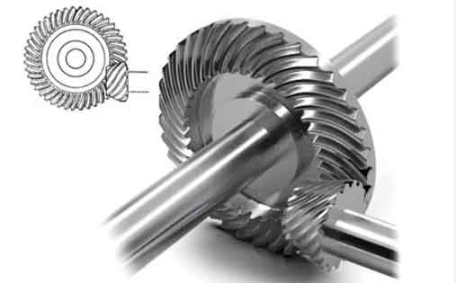
In the realm of mechanical transmission systems, spiral bevel gears play a pivotal role due to their ability to transmit motion between intersecting shafts with high efficiency, smooth operation, and reduced noise. Among these, zero-degree spiral bevel gears, characterized by a midpoint spiral angle of zero, are particularly valued in applications such as automotive drivetrains, marine propulsion, and heavy machinery. However, the complex geometry of their tooth surfaces, which are irregular and curved, poses significant challenges in design and manufacturing. Traditional methods often rely on specialized gear-cutting machines, such as face milling machines, to achieve the required precision. This study delves into the design methodology for zero-degree spiral bevel gears using the face milling method, leveraging spatial meshing principles and generative machining theory. Through computational programming in MATLAB and 3D modeling in Pro/ENGINEER (Pro/E), we develop accurate geometric models that facilitate transmission analysis and manufacturing processes. The integration of mathematical derivations, parameter optimization, and digital prototyping underscores the advancement in gear design, offering a robust framework for engineering applications. Throughout this article, the term ‘spiral bevel gears’ will be emphasized to highlight the focus on this gear type, with zero-degree variants as a specific case study.
The face milling method for manufacturing spiral bevel gears involves simulating a virtual gear, known as the generating gear or crown gear, on a machine tool’s cradle. During machining, a rotating cutter head, representing a tooth surface of this generating gear, engages with the gear blank in a coordinated motion to carve out the tooth slots. This generative process ensures that the tooth profiles conform to the desired meshing conditions. For zero-degree spiral bevel gears, the lack of spiral angle simplifies some aspects but complicates others, particularly in achieving proper tooth contact and strength. The design process begins with understanding the spatial kinematics and coordinate transformations inherent in gear machining. By deriving the tooth surface equations based on cutter geometry and machine settings, we can predict the gear’s performance and optimize its parameters. This approach not only enhances accuracy but also reduces reliance on physical prototypes, aligning with modern digital manufacturing trends. In the following sections, we will explore the theoretical foundations, mathematical formulations, and practical implementations, culminating in a comprehensive design framework for spiral bevel gears.
The core of designing spiral bevel gears lies in the derivation of tooth surface equations. These equations describe the geometry of the gear teeth in three-dimensional space, accounting for the machining process. For the face milling method, we start with the cutter profile, which is typically a conical surface defined by parameters such as cutter radius, blade angle, and tooth depth. Consider a dual-blade cutter used for machining the gear’s convex and concave sides. The cutter’s axial cross-section can be represented mathematically, and by rotating this profile, we obtain the cutter surface. Let $r_v$ denote the cutter radius, $\alpha$ the blade angle (often 20 degrees), $w$ the blade edge distance, $h_t$ the total tooth height, and $t$ a parameter along the cutter profile. The cutter surface equation in its local coordinate system $(X_t, Y_t, Z_t)$ is given by:
$$
\mathbf{r}_c(t, \theta) = \begin{cases}
X_t = (t + r_v) \cos \theta \\
Y_t = (t + r_v) \sin \theta \\
Z_t = f(t)
\end{cases}
$$
where $\theta$ is the rotation angle around the cutter axis, and $f(t)$ defines the profile shape. For instance, for the convex side (inner blade), $f(t)$ might be linear segments based on the blade angle. The unit normal vector $\mathbf{n}_c$ to this surface is derived from partial derivatives, essential for subsequent meshing analysis. To translate this cutter geometry into the gear tooth surface, we employ a series of coordinate transformations that mirror the machine tool setup. These transformations account for the radial and axial positions of the cutter, the cradle rotation, and the gear blank’s orientation. By combining these transformations, we obtain the tooth surface equation in the gear coordinate system, denoted as $\mathbf{r}_b(t, \theta, \phi_m)$, where $\phi_m$ is the generating gear’s rotation angle during machining.
The meshing condition between the generating gear and the gear blank is governed by the equation of contact, which ensures that the surfaces are tangent at each point of contact. This condition is expressed as:
$$
\mathbf{n}_b \cdot \mathbf{v}_{b,m} = 0
$$
where $\mathbf{n}_b$ is the unit normal vector of the tooth surface in the gear coordinate system, and $\mathbf{v}_{b,m}$ is the relative velocity between the gear blank and the generating gear. Solving this equation along with the tooth surface equation eliminates the parameter $\phi_m$, yielding a relation between $t$ and $\theta$ that defines the active tooth surface. For zero-degree spiral bevel gears, the simplicity in spiral angle often leads to symmetric equations, but the curvature adjustments for optimal contact patterns require careful parameter selection. The derivation involves matrix transformations, such as rotation and translation matrices, which encode the machine settings like cutter radial distance $R_c$, axial distance $A_c$, and machine root angle $\gamma$. Below, we present a summary of key parameters for a sample gear pair, illustrating the design inputs for spiral bevel gears.
| Parameter | Pinion (Small Gear) | Gear (Large Gear) |
|---|---|---|
| Number of Teeth | 42 | 15 |
| Module at Large End (mm) | 8 | 8 |
| Face Width (mm) | 52 | 52 |
| Pressure Angle (degrees) | 20 | 20 |
| Midpoint Spiral Angle (degrees) | 0 | 0 |
| Shaft Angle (degrees) | 90 | 90 |
To implement this mathematically, we use MATLAB for symbolic and numerical computations. The code defines the cutter profile, sets up transformation matrices, and solves the meshing equation iteratively. For example, the transformation from cutter coordinates to gear coordinates involves multiple steps: first to the cradle system, then to the machine system, and finally to the gear blank system. Each step is represented by a homogeneous transformation matrix $T_{ij}$, which combines rotation and translation. For the gear (large gear), the transformation chain is:
$$
\mathbf{r}_b = T_{b,a}(\phi) \cdot T_{a,m} \cdot T_{m,0}(\phi_m) \cdot T_{0,c} \cdot \mathbf{r}_c
$$
where $\phi = -i \phi_m$, with $i$ being the machine ratio (related to the gear ratio). The subscripts denote coordinate systems: $c$ for cutter, $0$ for cradle, $m$ for machine, $a$ for auxiliary, and $b$ for gear blank. The normal vector transforms similarly using the rotational parts of these matrices. By programming this in MATLAB, we compute points on the tooth surface by varying $t$ and $\theta$ within specified ranges. The range for $t$ is determined by the cutter profile limits, such as from $-h_t \tan \alpha – w/2$ to $h_t \tan \alpha + w/2$, while $\theta$ is constrained by the intersection of cutter and gear blank boundaries during machining. This intersection is visualized in a diagram where the cutter’s effective cutting zone overlaps with the gear’s cone dimensions, ensuring that only relevant surface points are generated. The computational output is a set of $(x, y, z)$ coordinates for each tooth surface, which can be exported for 3D modeling.
For the pinion (small gear), the process is analogous but often requires separate machining for convex and concave sides due to the use of single-blade cutters. The cutter parameters differ, as shown in the machine settings table below. These settings are critical for achieving the correct tooth geometry and contact pattern for spiral bevel gears. The face milling method allows for adjustments in parameters like cutter radius and blade angle to optimize performance, which is why detailed tables are essential in design.
| Parameter | Gear (Large) | Pinion Concave Side | Pinion Convex Side |
|---|---|---|---|
| Cutter Radius (mm) | 152.4 | 168.4 | 142.0 |
| Blade Angle (degrees) | 20 | 20 | 20 |
| Blade Edge Distance (mm) | 6.1 | 4.0 | 4.0 |
| Radial Cutter Position (mm) | 218.158 | 231.690 | 208.300 |
| Axial Cutter Position (degrees) | 44.3129 | 46.4719 | 42.9768 |
| Blank Installation Angle (degrees) | 66.2574 | 17.6136 | 17.6136 |
| Machine Ratio | 1.0618 | 2.9738 | 2.9738 |
Once the tooth surface points are computed, the next step is to create a 3D solid model. This is achieved by importing the point data into Pro/ENGINEER, a CAD software. The points are formatted into an IBLS (Interface Boundary Line Segment) file, which Pro/E can interpret to generate curves and surfaces. In the IBLS file, points are organized into curves representing cross-sections of the tooth surface. For example, each curve corresponds to a constant parameter line, and multiple curves are blended to form a continuous surface. Using Pro/E’s surfacing tools, such as boundary blend, we construct the tooth face, and then trim it with the gear blank boundaries to create a solid tooth slot. This process is repeated for all teeth via pattern operations, resulting in a complete gear model. The accuracy of this model relies on the density of computed points; finer meshes yield smoother surfaces but require more computational effort. For spiral bevel gears, ensuring proper curvature continuity is vital to avoid stress concentrations and noise in operation.
To validate the design, we assemble the pinion and gear models in Pro/E and perform motion simulation. This checks for interference, contact patterns, and kinematic behavior. The simulation confirms that the gears mesh smoothly without collisions, and the contact ellipse—a key indicator of load distribution—aligns with theoretical predictions. The use of digital prototypes reduces the need for physical testing, saving time and resources in the development of spiral bevel gears. Moreover, the model can be exported for finite element analysis (FEA) to assess strength and durability, or for CNC programming to guide actual machining. This integrated approach from theory to digital modeling exemplifies modern engineering practices for complex components like spiral bevel gears.
The mathematical derivation of tooth surfaces is central to this methodology. Let’s delve deeper into the equations for both gear and pinion. Starting with the cutter profile, we define it piecewise based on the blade segments. For the gear’s convex side, the profile function $f(t)$ in the cutter coordinate system can be expressed as:
$$
f(t) = \begin{cases}
-\frac{1}{\tan \alpha} \left( t + \frac{w}{2} \right), & -\frac{w}{2} \leq t < \frac{w}{2} \\
\text{other segments as per design}
\end{cases}
$$
After rotation, the cutter surface vector is $\mathbf{r}_c(t, \theta) = [X_t, Y_t, Z_t, 1]^T$. The transformation matrices involve rotations and translations. For instance, $T_{0,c}$ translates from cutter to cradle coordinates, incorporating the radial distance $R_c$ and axial distance $A_c$:
$$
T_{0,c} = \begin{bmatrix}
1 & 0 & 0 & R_c \cos A_c \\
0 & 1 & 0 & R_c \sin A_c \\
0 & 0 & 1 & 0 \\
0 & 0 & 0 & 1
\end{bmatrix}
$$
Subsequent matrices account for cradle rotation $\phi_m$ and gear blank rotation $\phi$. The meshing equation is derived from the relative velocity. In the gear coordinate system, the velocity of a point on the tooth surface relative to the generating gear is:
$$
\mathbf{v}_{b,m} = \frac{d\mathbf{r}_b}{d\tau} = \omega_m \frac{d\mathbf{r}_b}{d\phi_m}
$$
where $\omega_m$ is the angular velocity of the generating gear. Substituting into the contact equation yields a nonlinear equation in $t$, $\theta$, and $\phi_m$. Solving this numerically in MATLAB, we use iterative methods like Newton-Raphson to find valid $(t, \theta)$ pairs for given $\phi_m$. The resulting point cloud defines the tooth surface. To ensure full coverage, we sample $\phi_m$ over its range, which is determined by the gear blank’s cone angles and cutter engagement. Typically, $\phi_m$ ranges from $-\Phi$ to $\Phi$, where $\Phi$ is calculated from the gear geometry.
For the pinion, the derivation is similar but with different cutter parameters and transformation matrices due to its orientation. The machine ratio $i$ for the pinion is higher, reflecting its smaller number of teeth relative to the generating gear. This affects the relationship $\phi = -i \phi_m$, altering the surface curvature. The pinion’s tooth surfaces are often designed separately for concave and convex sides to optimize contact patterns, a common practice in spiral bevel gear design. The equations become:
$$
\mathbf{r}_{b,\text{pinion}} = T_{b,a}(\phi) \cdot T_{a,m} \cdot T_{m,0}(\phi_m) \cdot T_{0,c} \cdot \mathbf{r}_{c,\text{pinion}}
$$
where $\mathbf{r}_{c,\text{pinion}}$ is based on a single-blade cutter profile. The meshing condition is applied analogously. The complexity arises from the need to match the pinion and gear surfaces for conjugate action, ensuring smooth transmission of motion. This requires iterative adjustment of machine settings, which can be automated using optimization algorithms in MATLAB.
In practice, the design of spiral bevel gears involves trade-offs between geometric accuracy, manufacturing feasibility, and performance. The face milling method offers flexibility through parameters like cutter radius and blade angle. For zero-degree spiral bevel gears, the absence of spiral angle simplifies the calculation of some parameters but may necessitate compromises in load capacity or noise. Therefore, the design process often includes sensitivity analysis, where key parameters are varied to assess their impact on tooth contact pressure, bending stress, and transmission error. This can be facilitated by coupling the MATLAB computations with FEA software, creating a closed-loop design system. The tables below summarize additional design considerations for spiral bevel gears, highlighting parameters that influence performance.
| Parameter | Effect on Gear Performance | Typical Range |
|---|---|---|
| Cutter Radius | Affects tooth curvature and contact pattern | 100-200 mm |
| Blade Angle | Determines pressure angle and tooth strength | 15-25 degrees |
| Machine Ratio | Controls tooth profile shape and conjugation | 1.0-3.0 |
| Radial Cutter Position | Influences tooth depth and root geometry | 150-250 mm |
To illustrate the computational process, consider a MATLAB script snippet for solving the tooth surface points. We define symbolic variables for $t$, $\theta$, and $\phi_m$, set up the transformation matrices, and use a loop to compute points. The output is saved as a text file for Pro/E import. The accuracy of the model depends on the step sizes for $t$ and $\theta$; smaller steps yield more points but increase computation time. For a gear with 15 teeth, we might generate thousands of points per tooth to ensure a smooth surface. This point data is then used in Pro/E to create a solid model through the following steps: import points, create curves, blend surfaces, extrude the gear blank, and subtract the tooth slots. The resulting 3D model can be visualized and analyzed for any geometric discrepancies.
The advantages of this digital design approach for spiral bevel gears are manifold. It reduces the need for physical prototypes, accelerates the design cycle, and enables optimization for specific applications. For instance, in automotive differentials, zero-degree spiral bevel gears must transmit torque efficiently while minimizing noise; the digital model allows for simulation of noise-vibration-harshness (NVH) characteristics. Moreover, the integration with CNC machining ensures that the designed geometry can be manufactured accurately, bridging the gap between design and production. The face milling method, with its well-defined parameters, lends itself to such digital workflows, making it a preferred choice for high-precision spiral bevel gears.
In conclusion, the design of zero-degree spiral bevel gears based on the face milling method is a comprehensive process that combines theoretical mechanics, computational mathematics, and computer-aided design. By deriving tooth surface equations from cutter geometry and machine kinematics, we can predict gear behavior and optimize designs. The use of MATLAB for numerical solutions and Pro/E for 3D modeling provides a robust platform for creating accurate digital prototypes. This methodology not only enhances the design of spiral bevel gears but also supports advancements in manufacturing technologies. Future work may involve extending this approach to helical or hypoid gears, incorporating more complex material models, or integrating with additive manufacturing for customized gear production. Ultimately, the goal is to advance the engineering of spiral bevel gears for more efficient and reliable mechanical systems.
To further elaborate on the mathematical details, let’s consider the coordinate transformation matrices in full. For the gear, the transformation from cutter coordinates $(X_c, Y_c, Z_c)$ to gear blank coordinates $(X_b, Y_b, Z_b)$ involves several steps. First, the cutter coordinates are transformed to the cradle system $(X_0, Y_0, Z_0)$ with a translation and rotation based on the cutter position. This is represented by matrix $T_{0,c}$, which includes terms for radial distance $R_c$ and axial angle $A_c$. Next, the cradle system rotates by angle $\phi_m$ to account for the generating motion, yielding the machine system $(X_m, Y_m, Z_m)$ via matrix $T_{m,0}(\phi_m)$. Then, the machine system is translated to an auxiliary system $(X_a, Y_a, Z_a)$ using matrix $T_{a,m}$, which incorporates the gear blank offset. Finally, the auxiliary system rotates by the gear blank angle $\phi$ to produce the gear blank coordinates with matrix $T_{b,a}(\phi)$. The composite transformation is:
$$
\mathbf{r}_b = T_{b,a}(\phi) \cdot T_{a,m} \cdot T_{m,0}(\phi_m) \cdot T_{0,c} \cdot \mathbf{r}_c
$$
Each matrix is a 4×4 homogeneous transformation. For example, $T_{m,0}(\phi_m)$ is a rotation matrix around the cradle axis:
$$
T_{m,0}(\phi_m) = \begin{bmatrix}
\cos \phi_m & -\sin \phi_m & 0 & 0 \\
\sin \phi_m & \cos \phi_m & 0 & 0 \\
0 & 0 & 1 & 0 \\
0 & 0 & 0 & 1
\end{bmatrix}
$$
The normal vector transformation uses the rotational submatrices (3×3) of these matrices, denoted as $L_{ij}$. Thus, $\mathbf{n}_b = L_{b,a}(\phi) \cdot L_{a,m} \cdot L_{m,0}(\phi_m) \cdot L_{0,c} \cdot \mathbf{n}_c$. The meshing equation then becomes a scalar equation that can be solved numerically. In MATLAB, we set up these matrices symbolically, compute derivatives for velocity, and use a solver to find solutions. The results are point coordinates that define the tooth surface for spiral bevel gears.
For the pinion, similar transformations apply, but with different angles and distances. The machine ratio $i$ links the pinion rotation to the cradle rotation: $\phi_{\text{pinion}} = -i \phi_m$. This ratio is derived from the gear ratio and affects the tooth profile. The cutter for the pinion may have a different radius and blade setting, as shown in Table 2. The derivation of pinion tooth surfaces follows the same principles, emphasizing the importance of accurate parameter selection for conjugate action in spiral bevel gears.
In terms of practical implementation, the MATLAB code outputs a file with point coordinates. In Pro/E, these points are imported to create datum points, which are then connected into splines. These splines serve as boundaries for surface creation. Using the boundary blend tool, we generate a surface that fits these splines, ensuring tangency continuity where needed. This surface is then trimmed with the gear blank solid to create a tooth slot. Pattern this slot around the axis to form all teeth, and then add features like hubs or keyways to complete the gear model. The process is similar for both gear and pinion, resulting in an assembly that can be tested for interference and motion.
The design methodology presented here for spiral bevel gears is not limited to zero-degree variants; it can be adapted for gears with non-zero spiral angles by adjusting the transformation matrices to include spiral angle components. The face milling method is versatile, and the mathematical framework remains largely the same. However, for zero-degree spiral bevel gears, the simplification in spiral angle reduces some complexity in equations, making it an ideal starting point for understanding gear design. The repeated emphasis on spiral bevel gears throughout this article underscores their significance in mechanical engineering and the need for precise design tools.
To summarize, this article has detailed a comprehensive approach to designing zero-degree spiral bevel gears using the face milling method. From theoretical foundations involving spatial meshing and coordinate transformations to practical steps in MATLAB and Pro/E, we have covered the entire process. The use of tables and equations highlights the methodical nature of gear design, while the digital modeling aspects align with modern engineering practices. The integration of these elements facilitates the creation of accurate and functional spiral bevel gears for various applications, contributing to advancements in transmission technology. As industries demand higher performance and efficiency, such design methodologies will continue to evolve, further enhancing the capabilities of spiral bevel gears in complex mechanical systems.