
Hypoid gears represent a critical and sophisticated class of gear drives extensively utilized in automotive, aerospace, marine, and heavy machinery applications. Their distinguishing features, including high load capacity, compact design, and the ability to transmit motion between non-intersecting and non-parallel shafts with a substantial offset, make them indispensable for power transmission in confined spaces. The manufacturing process of hypoid gears is complex, with the Head Cutter Tilt (HFT) method, also known as the Formate (pinion)/Generate (gear) method, being a predominant technique. Accurately modeling the tooth surfaces, including the vital fillet transition regions, is foundational for analyzing their meshing behavior, contact patterns, transmission error, and dynamic response under load. This article delves into a comprehensive methodology for the digital modeling and analysis of the time-varying meshing characteristics of hypoid gears manufactured via the HFT process.
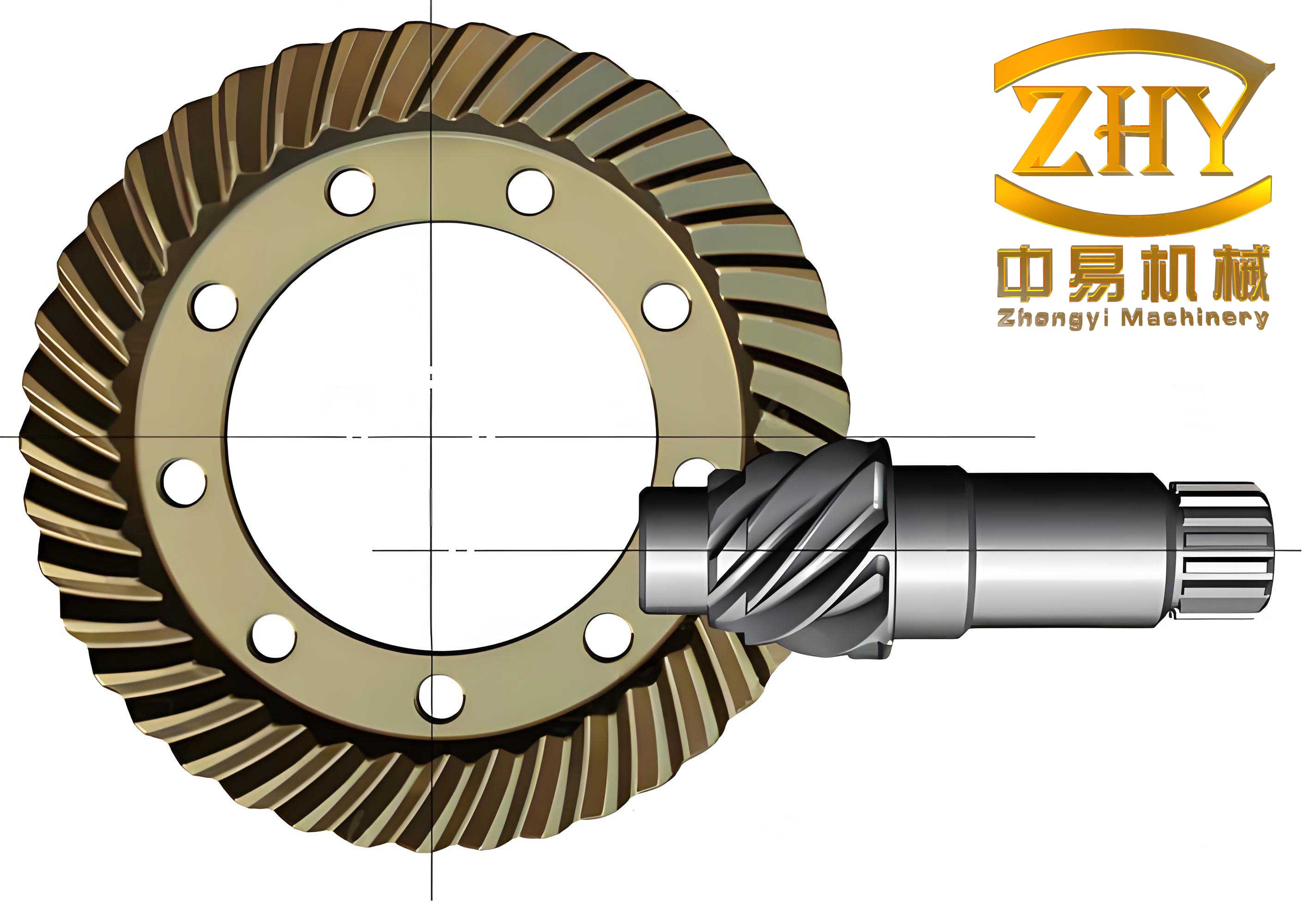
The core of accurate modeling lies in mathematically simulating the machining kinematics of a cradle-style hypoid gear generator. The process involves the coordinated motion of the cutter head, the workpiece (gear or pinion blank), and the cradle. For the gear member, which is typically cut using a Formate (non-generating) process with a double-sided cutter, the relative motion is simpler. For the pinion, the HFT method introduces additional complexities with cutter tilt and swivel motions to achieve the desired localized bearing contact. The mathematical framework employs homogeneous coordinate transformation matrices to map a point on the cutting tool surface to its final position on the finished tooth surface in the workpiece coordinate system.
1. Mathematical Modeling of the Machining Process and Tooth Surface Generation
The generation of tooth surfaces for hypoid gears is governed by the envelope theory, where the family of surfaces generated by the moving cutting tool envelopes the final tooth surface. Defining a series of coordinate systems attached to the machine tool components is essential.
1.1 Coordinate Systems and Transformation for the Gear (Formate Cutting)
For the gear, cut via the Formate method, the primary coordinate systems and their associated machine settings are defined below. The transformation chain from the cutter coordinate system \( S_{t2} \) to the gear blank coordinate system \( S_2 \) is constructed via intermediate frames.
| Coordinate System | Definition | Key Associated Parameters |
|---|---|---|
| \( S_{t2}(O_{t2}, X_{t2}, Y_{t2}, Z_{t2}) \) | Cutter Head Frame | Fixed to the gear cutter head. |
| \( S_{g}(O_{g}, X_{g}, Y_{g}, Z_{g}) \) | Cutter Rotation Frame | Cutter rotation angle \( \theta_g \). |
| \( S_{a2}(O_{a2}, X_{a2}, Y_{a2}, Z_{a2}) \) | Cradle Radial/Swivel Frame | Radial distance \( S_{r2} \), swivel angle \( q_2 \). |
| \( S_{b2}(O_{b2}, X_{b2}, Y_{b2}, Z_{b2}) \) | Sliding Base Frame | Machine center to back (\( X_{B2} \)). |
| \( S_{c2}(O_{c2}, X_{c2}, Y_{c2}, Z_{c2}) \) | Machine Bed Frame | Vertical offset (\( E_2 \)). |
| \( S_{d2}(O_{d2}, X_{d2}, Y_{d2}, Z_{d2}) \) | Root Angle Frame | Machine root angle (\( \delta_{M2} \)). |
| \( S_{2}(O_{2}, X_{2}, Y_{2}, Z_{2}) \) | Gear Blank Frame | Axial position (\( X_2 \)). |
The position vector of a point \( G \) on the inner (convex side) cutting blade in the cutter frame \( S_g \) is given by:
$$ \mathbf{r}_g = \begin{bmatrix} (r_G – u_g \sin \alpha_2) \cos \theta_g \\ (r_G – u_g \sin \alpha_2) \sin \theta_g \\ -u_g \cos \alpha_2 \\ 1 \end{bmatrix} $$
where \( u_g \) is the profile parameter (length along the cutting edge), \( \theta_g \) is the rotation parameter of the cutter, \( \alpha_2 \) is the tool pressure angle, and \( r_G = r_0 \pm P_{W2}/2 \) is the point radius ( \( r_0 \) is the nominal cutter radius, \( P_{W2} \) is the point width, ‘-‘ for inner blade, ‘+’ for outer blade). The unit normal vector at this point is:
$$ \mathbf{n}_g = \frac{\partial \mathbf{r}_g}{\partial \theta_g} \times \frac{\partial \mathbf{r}_g}{\partial u_g} \bigg/ \left\| \frac{\partial \mathbf{r}_g}{\partial \theta_g} \times \frac{\partial \mathbf{r}_g}{\partial u_g} \right\| = \begin{bmatrix} -\cos \alpha_2 \cos \theta_g \\ -\cos \alpha_2 \sin \theta_g \\ \sin \alpha_2 \end{bmatrix} $$
The transformation to the gear blank coordinate system is achieved through the homogeneous transformation matrix \( \mathbf{M}_{gs2} \):
$$ \mathbf{M}_{gs2} = \mathbf{Trans}(-X_2, 0, 0) \cdot \mathbf{Rot}_y(\delta_{M2}) \cdot \mathbf{Trans}(0, E_2, -X_{B2}) \cdot \mathbf{Trans}(S_{r2}\cos q_2, S_{r2}\sin q_2, 0) $$
The position vector \( \mathbf{r}_2 \) and the unit normal vector \( \mathbf{n}_2 \) in the gear coordinate system \( S_2 \) are then:
$$ \mathbf{r}_2 = \mathbf{M}_{gs2} \cdot \mathbf{r}_g, \quad \mathbf{n}_2 = \mathbf{L}_{gs2} \cdot \mathbf{n}_g $$
where \( \mathbf{L}_{gs2} \) is the 3×3 rotational sub-matrix extracted from \( \mathbf{M}_{gs2} \). To obtain discrete points on the tooth surface, a grid is defined in the gear axial section. For each grid point with coordinates \( (x_{L2}^i, y_{L2}^i) \), the corresponding surface parameters \( (u_g^i, \theta_g^i) \) are solved from the system:
$$ \begin{cases} x_2^i(u_g, \theta_g) = x_{L2}^i \\ (y_2^i(u_g, \theta_g))^2 + (z_2^i(u_g, \theta_g))^2 = (y_{L2}^i)^2 \end{cases} $$
1.2 Gear Fillet (Root Transition) Surface
The fillet surface is generated by the rounded tip of the cutting tool. Its equation is derived similarly, but the cutting edge is defined by a circular arc of radius \( r_{gf} \). In the cutter frame \( S_{t2} \), the vector for the fillet is parameterized by an angle \( \gamma_g \):
$$ \mathbf{r’}_{t2} = \begin{bmatrix} r_G – u_{g0} \sin \alpha_2 \pm r_{gf}\cos \alpha_2 \mp r_{gf}\sin \gamma_g \\ 0 \\ – u_{g0} \cos \alpha_2 \mp r_{gf}\sin \alpha_2 + r_{gf}\cos \gamma_g \\ 1 \end{bmatrix} $$
where \( u_{g0} \) is the parameter at the tangency point between the main cutting edge and the fillet arc. Applying the same transformation chain \( \mathbf{M}_{gs2} \) yields the fillet surface \( \mathbf{r’}_2(u_g, \theta_g, \gamma_g) \) in the gear coordinate system.
1.3 Coordinate Systems and Transformation for the Pinion (HFT Generating)
Modeling the pinion tooth surface is more intricate due to the generating roll motion and the additional cutter tilt and swivel settings. The primary coordinate systems are defined as follows:
| Coordinate System | Definition | Key Associated Parameters |
|---|---|---|
| \( S_{t1}(O_{t1}, X_{t1}, Y_{t1}, Z_{t1}) \) | Pinion Cutter Head Frame | Fixed to the pinion cutter. |
| \( S_{p}(O_{p}, X_{p}, Y_{p}, Z_{p}) \) | Pinion Cutter Rotation Frame | Cutter rotation angle \( \theta_p \). |
| \( S_{a1}(O_{a1}, X_{a1}, Y_{a1}, Z_{a1}) \) | Cutter Tilt Frame | Tilt angle \( i_1 \). |
| \( S_{b1}(O_{b1}, X_{b1}, Y_{b1}, Z_{b1}) \) | Cutter Swivel Frame | Swivel angle \( j_1 \). |
| \( S_{c1}(O_{c1}, X_{c1}, Y_{c1}, Z_{c1}) \) | Radial Distance Frame | Radial setting \( S_{r1} \). |
| \( S_{d1}(O_{d1}, X_{d1}, Y_{d1}, Z_{d1}) \) | Cradle Frame | Swivel angle \( q_1 \). |
| \( S_{e1}(O_{e1}, X_{e1}, Y_{e1}, Z_{e1}) \) | Machine Bed Frame | Vertical offset (\( E_1 \)). |
| \( S_{f1}(O_{f1}, X_{f1}, Y_{f1}, Z_{f1}) \) | Sliding Base Frame | Machine center to back (\( X_{B1} \)). |
| \( S_{g1}(O_{g1}, X_{g1}, Y_{g1}, Z_{g1}) \) | Root Angle Frame | Machine root angle (\( \delta_{M1} \)). |
| \( S_{h1}(O_{h1}, X_{h1}, Y_{h1}, Z_{h1}) \) | Axial Position Frame | Axial setting (\( X_1 \)). |
| \( S_{1}(O_{1}, X_{1}, Y_{1}, Z_{1}) \) | Pinion Blank Frame | Blank rotation angle \( \phi_1 \). |
The position vector of a point \( P \) on the pinion cutter (e.g., outer blade for concave side) in \( S_p \) is:
$$ \mathbf{r}_p = \begin{bmatrix} (r_P + u_p \sin \alpha_1) \cos \theta_p \\ (r_P + u_p \sin \alpha_1) \sin \theta_p \\ -u_p \cos \alpha_1 \\ 1 \end{bmatrix} $$
where \( r_P \) is the point radius for the pinion cutter. The unit normal \( \mathbf{n}_p \) is derived accordingly. The comprehensive transformation matrix \( \mathbf{M}_{ps1} \) from \( S_p \) to \( S_1 \) incorporates all machine motions:
$$ \mathbf{M}_{ps1} = \mathbf{Trans}(-X_1,0,0)\mathbf{Rot}_x(\phi_1)\mathbf{Rot}_y(\delta_{M1})\mathbf{Trans}(0,E_1,-X_{B1})\mathbf{Rot}_z(q_1)\mathbf{Trans}(S_{r1},0,0)\mathbf{Rot}_z(j_1)\mathbf{Rot}_x(i_1) $$
Thus, \( \mathbf{r}_1 = \mathbf{M}_{ps1} \cdot \mathbf{r}_p \) and \( \mathbf{n}_1 = \mathbf{L}_{ps1} \cdot \mathbf{n}_p \). Unlike the gear, the pinion surface generation involves a conjugate relationship between the generating gear (cradle) and the workpiece. This is enforced by the equation of meshing:
$$ \mathbf{n}^{(e1)}_p \cdot \mathbf{v}^{(e1)}_{p} = 0 $$
where \( \mathbf{n}^{(e1)}_p \) is the unit normal vector of the cutter surface expressed in the machine bed frame \( S_{e1} \), and \( \mathbf{v}^{(e1)}_{p} \) is the relative velocity between the cutter and the pinion blank in the same frame. The cradle rotation angle \( \phi_c \) is related to the pinion blank rotation \( \phi_1 \) through the machine ratio \( i_{01} = \omega_w / \omega_c = \phi_1 / \phi_c \). To solve for the pinion tooth surface coordinates \( (x_1^i, y_1^i, z_1^i) \) corresponding to axial section grid points \( (x_{L1}^i, y_{L1}^i) \), the following system of three equations with three unknowns \( (u_p, \theta_p, \phi_1) \) is solved numerically:
$$ \begin{cases} x_1(u_p, \theta_p, \phi_1) = x_{L1}^i \\ (y_1(u_p, \theta_p, \phi_1))^2 + (z_1(u_p, \theta_p, \phi_1))^2 = (y_{L1}^i)^2 \\ \mathbf{n}^{(e1)}_p(u_p, \theta_p) \cdot \mathbf{v}^{(e1)}_{p}(u_p, \theta_p, \phi_1) = 0 \end{cases} $$
1.4 3D Digital Model Assembly
Using the solved discrete point clouds for both the active tooth surfaces and the fillet surfaces of the gear and pinion, non-uniform rational B-spline (NURBS) surfaces can be fitted. These surfaces are then used to perform a Boolean subtraction operation from solid gear blanks, resulting in precise 3D digital models of the hypoid gears. The design and machine settings for an example gear drive are summarized below.
| Parameter | Pinion (Drive, Left Hand) | Gear (Driven, Right Hand) |
|---|---|---|
| Number of Teeth | 10 | 41 |
| Module (mm) | 4.741 | |
| Shaft Angle (°) | 90 | |
| Offset (mm) | -31.8 (Pinion below gear center) | |
| Face Width (mm) | 33.637 | 28 |
| Spiral Angle (°) | 49.9833 | 29.0000 |
| Parameter | Value |
|---|---|
| Cutter Nominal Diameter (in) | 7.5 |
| Outer Blade Pressure Angle (°) | -24 |
| Inner Blade Pressure Angle (°) | 17 |
| Point Width (in) | 0.09 |
| Tip Radius (in) | 0.04 |
| Radial Setting \( S_{r2} \) (mm) | 41.11 |
| Machine Root Angle \( \delta_{M2} \) (°) | 68.1333 |
| Parameter | Concave Side (Outer Blade) | Convex Side (Inner Blade) |
|---|---|---|
| Blade Pressure Angle \( \alpha_1 \) (°) | 14 | -31 |
| Point Radius \( r_P \) (mm) | 92.456 | 97.917 |
| Tip Radius (in) | 0.0025 | |
| Radial Setting \( S_{r1} \) (mm) | 89.8950 | 93.5458 |
| Tilt Angle \( i_1 \) (°) | 21.2513 | 18.8262 |
| Swivel Angle \( j_1 \) (°) | -19.6319 | -34.2973 |
| Machine Ratio \( i_{01} \) | 3.87250 | 4.03515 |
2. Tooth Contact Analysis (TCA)
Tooth Contact Analysis is performed to predict the unloaded meshing behavior of the theoretically generated hypoid gears, including the transmission error (TE) and the contact pattern.
2.1 Mathematical Model for Meshing
The gear and pinion tooth surfaces, originally defined in their respective coordinate systems \( S_2 \) and \( S_1 \), must be represented in a fixed meshing coordinate system \( S_H \). Assuming at time \( t \), the pinion has rotated by an angle \( \phi_{h1} \) and the gear by \( \phi_{h2} \) from their initial assembly positions, the position vectors in \( S_H \) are:
$$ \mathbf{r}_1^H = \mathbf{Rot}_x(\phi_{h1}) \cdot \mathbf{r}_1, \quad \mathbf{n}_1^H = \mathbf{Rot}_x(\phi_{h1}) \cdot \mathbf{n}_1 $$
$$ \mathbf{r}_2^H = \mathbf{Trans}(0, E, 0) \mathbf{Rot}_y(\Sigma) \mathbf{Rot}_x(\phi_{h2}) \cdot \mathbf{r}_2, \quad \mathbf{n}_2^H = \mathbf{Rot}_y(\Sigma) \mathbf{Rot}_x(\phi_{h2}) \cdot \mathbf{n}_2 $$
where \( \Sigma \) is the shaft angle (90°) and \( E \) is the offset. At the point of instantaneous contact, the following conditions must be satisfied:
$$ \begin{cases} \mathbf{r}_1^H(u_p, \theta_p, \phi_1) = \mathbf{r}_2^H(u_g, \theta_g) \\ \mathbf{n}_1^H(u_p, \theta_p, \phi_1) = \mathbf{n}_2^H(u_g, \theta_g) \end{cases} $$
This system effectively contains five independent scalar equations. The unknowns are the four surface parameters \( (u_p, \theta_p, u_g, \theta_g) \) and the two rotation angles \( (\phi_{h1}, \phi_{h2}) \). However, for the pinion, \( u_p \) is not independent and can be expressed as a function of \( \theta_p \) and \( \phi_1 \) via the equation of meshing from the generation process. By prescribing the pinion rotation angle \( \phi_{h1} \) as an input, the system can be solved numerically for the remaining five unknowns, yielding one contact point. Iterating \( \phi_{h1} \) over the mesh cycle provides the path of contact and the corresponding gear rotation \( \phi_{h2} \).
2.2 Static Transmission Error and Unloaded Contact Pattern
The static transmission error (STE), a primary source of vibration and noise in hypoid gears, is calculated from the solved rotation angles:
$$ \delta(\phi_{h1}) = (\phi_{h2} – \phi_{h2}^0) – \frac{z_1}{z_2} (\phi_{h1} – \phi_{h1}^0) $$
where \( z_1, z_2 \) are the numbers of teeth, and \( \phi_{h1}^0, \phi_{h2}^0 \) are the initial angles of engagement. The unloaded contact pattern is determined by calculating the instantaneous contact ellipse at each calculated point of contact, based on the principal curvatures and relative normal curvature of the two surfaces. For the example gear pair, the TCA results typically show a controlled, localized elliptical contact patch positioned in the mid-face and mid-flank region under no load, with a parabolic function-like STE curve of minimal amplitude, indicating a well-designed pair of hypoid gears.
3. Loaded Tooth Contact Analysis (LTCA) and Time-Varying Meshing Characteristics
While TCA provides insight into the unloaded behavior, the actual performance of hypoid gears under operating loads is characterized by significant changes in contact patterns, transmission error, load sharing, and mesh stiffness. Finite Element Analysis (FEA) is a powerful tool for conducting Loaded Tooth Contact Analysis.
3.1 Finite Element Model Setup
The 3D digital models of the pinion and gear are imported into a pre-processor (e.g., HyperMesh) for meshing. To balance accuracy and computational cost, a multi-slice modeling approach is often used: a full-tooth model for the pinion and a sector model (e.g., 18 teeth) for the gear. The mesh is refined in the potential contact zones and fillet regions. The model is then solved in a commercial FEA package like ABAQUS using implicit static analysis. Key setup parameters include:
| Parameter | Value/Specification |
|---|---|
| Material (Steel) | Young’s Modulus = 209 GPa, Poisson’s Ratio = 0.3, Density = 7850 kg/m³ |
| Contact Definition | Surface-to-surface, finite sliding, “Hard” contact normal behavior, friction coefficient = 0.1 |
| Element Type | C3D8R (8-node linear brick, reduced integration) |
| Boundary Conditions | Pinion shaft center: Coupled to reference point with prescribed rotation. Gear shaft center: Coupled to reference point with applied torque. Fixed axial and radial displacements at both reference points. |
| Analysis Steps | Initial step for contact stabilization, followed by a static step applying rotation and torque. |
3.2 Analysis of Time-Varying Meshing Parameters
The FEA solution is post-processed to extract time-varying (or more precisely, rotation-angle-varying) parameters over a complete mesh cycle. These parameters are crucial for understanding the dynamic behavior of hypoid gears.
Dynamic Meshing Force: The total contact force between the gear and pinion fluctuates periodically with the mesh frequency. Its amplitude is highly sensitive to the applied load.
Loaded Transmission Error (LTE): Under load, tooth deflections alter the kinematic relationship. The LTE is calculated from the difference between the actual output (gear) rotation and the ideal rigid-body rotation based on the input. Its waveform and amplitude are strong functions of load:
$$ \text{LTE}(\phi_{h1}) = \phi_{h2}^{\text{(FEA)}} – \phi_{h2}^{\text{(ideal)}} $$
Time-Varying Mesh Stiffness (TVMS): This is a fundamental excitation parameter in gear dynamics. For hypoid gears, it can be computed from the FEA results as the ratio of the total meshing force to the total deflection along the line of action (or its effective component):
$$ k_m(\phi_{h1}) = \frac{F_n(\phi_{h1})}{\delta_n(\phi_{h1})} $$
where \( F_n \) is the normal contact force and \( \delta_n \) is the composite normal deflection of the mating teeth, which can be derived from the LTE and the base circle radii. The TVMS curve for hypoid gears exhibits a complex, asymmetric shape due to the changing contact conditions across the face width.
Load Distribution and Contact Pressure: The contact ellipse deforms and spreads under load. The contact pattern shifts towards the heel (outer end) and toe (inner end) and expands, potentially covering most of the active profile at high loads. The maximum contact pressure increases with the applied torque.
Actual Contact Ratio: The number of tooth pairs in contact varies during the mesh cycle. Under light loads, the theoretical contact ratio may not be fully realized due to small deflections. As load increases, the increased tooth deflection allows earlier engagement and later separation, effectively increasing the actual contact ratio. This parameter stabilizes at higher loads.
3.3 Results and Discussion for the Example Hypoid Gears
Performing LTCA across a range of torques (e.g., from 100 Nm to 6000 Nm) on the gear for a constant pinion speed reveals significant trends:
Contact Pattern Evolution: At low torque, the contact patch is small and located centrally. As torque increases, the patch elongates along the lengthwise direction and expands toward the heel and toe ends. At the rated load, it should ideally cover a substantial portion of the tooth surface without reaching the edges. For the modeled hypoid gears, the start of contact typically shifts towards the heel with increasing load.
Transmission Error and Mesh Stiffness Behavior: The amplitude of the LTE fluctuation generally increases with load initially due to larger elastic deflections. However, after a certain load level, the amplitude may decrease as the contact spreads and the load sharing becomes more uniform. The TVMS curve becomes markedly asymmetric. With increasing load, the stiffness peak often occurs earlier in the mesh cycle. This is attributed to the contact shift towards the heel, where the effective tooth thickness is greater, making the tooth pair stiffer at that particular engagement position. The following table summarizes the qualitative influence of increasing load on key parameters:
| Meshing Parameter | Trend with Increasing Load | Primary Reason |
|---|---|---|
| Meshing Force Amplitude | Increases proportionally | Direct result of applied torque. |
| Loaded Transmission Error Amplitude | Increases, then may stabilize or decrease | Initial dominance of deflection, later improved load sharing. |
| Mesh Stiffness Peak Value & Shape | Increases; curve becomes asymmetric, peak shifts earlier | Contact zone moves to stiffer heel region; nonlinear load-deflection. |
| Contact Patch Size & Location | Expands significantly; shifts towards heel/toe | Tooth bending and local Hertzian deformation. |
| Maximum Contact Pressure | Increases sub-linearly | Pressure increases with sqrt(Load/Contact Area). |
| Actual Contact Ratio | Increases, approaching theoretical limit | Increased deflection enables earlier engagement/later recess. |
The analysis clearly shows that the meshing behavior of hypoid gears is highly nonlinear and load-dependent. The transition in LTE amplitude suggests there may be an optimal load range for minimal dynamic excitation. The pronounced asymmetry in TVMS is a key differentiator from parallel axis gears and must be accounted for in dynamic models of hypoid gear systems. Furthermore, the load sensitivity of the actual contact ratio in the low-torque regime highlights the importance of considering variable load sharing in the dynamic analysis of lightly loaded hypoid gear drives.
4. Conclusion
A comprehensive methodology for the digital modeling and analysis of hypoid gears has been presented, encompassing the mathematical simulation of the HFT machining process, precise tooth surface and fillet generation, unloaded Tooth Contact Analysis, and detailed Loaded Tooth Contact Analysis via the Finite Element Method. The accurate modeling of the machining kinematics using homogeneous coordinate transformations is fundamental to obtaining a truthful digital twin of the physical gears. The subsequent TCA and LTCA provide invaluable insights into the static and dynamic performance indicators. The results demonstrate that critical meshing parameters such as dynamic meshing force, loaded transmission error, time-varying mesh stiffness, and actual contact ratio exhibit significant and nonlinear dependence on the applied load. Notably, the loaded transmission error and mesh stiffness curves develop a distinct asymmetric character as the load increases, a direct consequence of the complex contact kinematics and load-induced deflections in hypoid gears. These findings and the established modeling framework provide a solid basis for the advanced analysis of transmission characteristics, dynamic behavior, noise-vibration-harshness (NVH) performance, and durability optimization of hypoid gear drives in demanding applications.