
In modern machinery, gear transmission stands as one of the most prevalent mechanical drive systems, extensively utilized across industries such as automotive, aerospace, marine, and heavy machinery. The advantages of gear drives include accurate and wide transmission ratios, high circumferential speeds, substantial power transmission capabilities, excellent efficiency, long service life, and compact design. However, they are not without drawbacks, notably vibration and noise generation, which can induce dynamic loads. Currently, high-speed rotating gears are widely employed in aerospace transmission systems, where circumferential speeds often reach 70–120 m/s, and transmitted power levels are significant. Consequently, mitigating vibration during gear operation and reducing damage to gears and mechanical systems is of paramount importance. Studies indicate that unbalance is among the most common causes of machinery failure, with approximately 50% of fault-related shutdowns directly attributable to unbalance, leading to issues like bearing damage, bearing housing cracks, shaft deformation, and gear scuffing. Therefore, in advanced transmission devices, critical high-speed rotating gears are subject to stringent dynamic balancing requirements.
From my perspective as an engineer specializing in rotary machinery, the dynamic balancing of gear shafts is not merely a supplementary process but a fundamental aspect of ensuring reliability and performance. In this article, I will delve into the principles, methods, and applications of dynamic balancing for gear shafts, emphasizing practical insights and calculations. The term “gear shaft” will be frequently referenced, as it represents a core component in many rotating systems where unbalance can have cascading effects. Through detailed explanations, formulas, and tables, I aim to provide a comprehensive guide that underscores the importance of precision in balancing procedures.
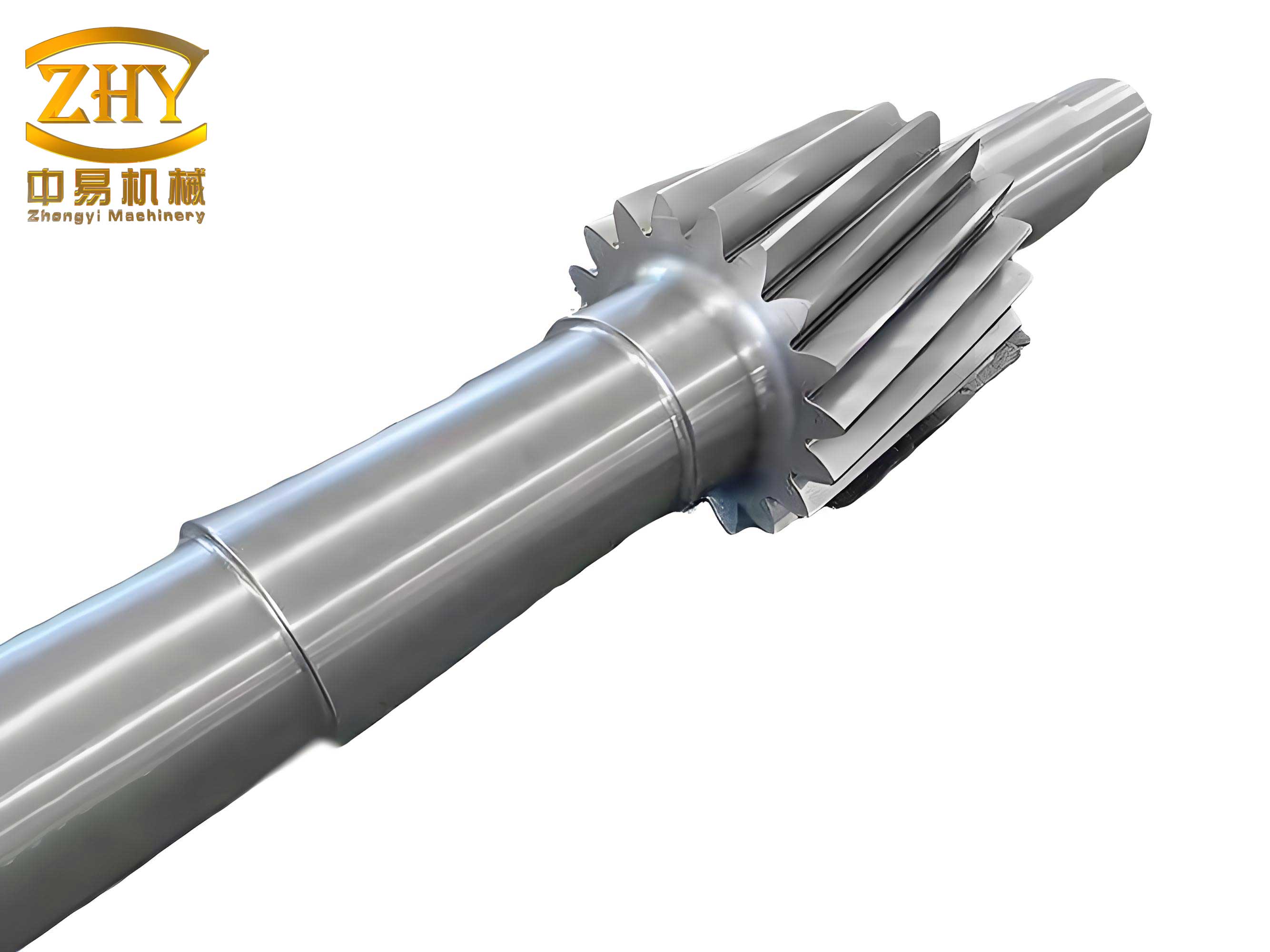
Ideally, a gear shaft is symmetric about its rotational axis. However, due to factors such as design limitations, material inconsistencies, manufacturing tolerances, and alterations in balance during operation, practical gear shafts always exhibit some degree of asymmetry, resulting in unbalance. Consider a single unbalanced mass point on a gear shaft with mass \(m\) located at a distance \(r\) from the axis of rotation. The centrifugal force \(F\) generated by this mass during rotation is given by:
$$F = m r \omega^2$$
where \(\omega\) is the angular velocity in radians per second. For a specific rotating gear shaft, \(m\) and \(r\) are constants, making the centrifugal force proportional to \(\omega^2\). The product \(m r\) serves as the proportionality constant and is defined as the unbalance amount \(U\), expressed as:
$$U = m r$$
Thus, the centrifugal force is linearly related to the unbalance amount \(U\). In high-speed rotating machinery, the unit of unbalance is typically gram-millimeters (g·mm). Unbalance is a vector quantity, possessing both magnitude and direction. In engineering practice, it is often represented as:
$$U = |U| \angle \theta$$
For example, \(U = 120 \, \text{g·mm} \angle 60^\circ\) indicates an unbalance magnitude of 120 g·mm at an angular position of 60° relative to a reference. This vector nature is crucial when correcting unbalance in gear shafts, as it influences the placement of correction masses.
For rigid rotors like gear shafts, two correction planes are sufficient to achieve balance. Provided the balancing system is sufficiently sensitive, test speeds need not be excessively high to expose and correct unbalance. Typically, a relatively low balancing speed (compared to operational speeds) can be selected, ensuring that the gear shaft rotates smoothly with uniform force distribution at both support points. The correction of unbalance involves adding or removing mass in these planes. Correction methods are categorized into two types: adding weight (positive correction) and removing weight (negative correction). Adding weight is often preferred for its process convenience; after balancing, correction masses are securely attached to the component, and adjustments during operation are straightforward. Conversely, removing weight is more tedious, requiring gradual material removal opposite the trial weight location until balance is achieved. This iterative process is time-consuming and less verifiable, as the exact amount removed is difficult to quantify. Despite these drawbacks, in sectors demanding high safety, reliability, and precision—such as aerospace—weight removal is commonly used for gear shaft dynamic balancing to avoid additional attached masses that could detach under high stresses.
The quality of gear dynamic balancing is assessed using the balance quality grade \(G\), which is expressed in millimeters per second (mm/s). It is derived from the product of the permissible specific unbalance \(e_{\text{per}}\) (in micrometers, μm) and the maximum operational angular velocity \(\omega\) (in rad/s), divided by 1000:
$$G = \frac{e_{\text{per}} \omega}{1000}$$
Alternatively, \(G\) can be related to the permissible residual unbalance \(U_{\text{per}}\) (in g·mm) and the rotor mass \(m\) (in kg). Since \(e_{\text{per}} = U_{\text{per}} / m\) (with \(e_{\text{per}}\) in μm, noting that 1 g·mm/kg = 1 μm), the formula becomes:
$$G = \frac{U_{\text{per}} \omega}{1000 \, m}$$
where \(\omega = 2 \pi n / 60\) for rotational speed \(n\) in revolutions per minute (r/min). Common balance quality grades include G2.5, G6.3, G16, and G40, selected based on application requirements. To illustrate, consider a gear shaft with mass \(m = 10 \, \text{kg}\) operating at \(n = 30000 \, \text{r/min}\). The angular velocity is \(\omega = 2 \pi \times 30000 / 60 \approx 3141.59 \, \text{rad/s}\). For a balance quality grade of G6.3, the permissible specific unbalance \(e_{\text{per}}\) can be calculated from \(G = e_{\text{per}} \omega / 1000\), yielding \(e_{\text{per}} = 1000 G / \omega \approx 2.00 \, \mu\text{m}\). Then, the permissible residual unbalance is \(U_{\text{per}} = m \times e_{\text{per}} = 10 \times 2.00 = 20.0 \, \text{g·mm}\). Table 1 summarizes calculations for different balance quality grades for this gear shaft example.
| Balance Quality Grade \(G\) (mm/s) | Angular Velocity \(\omega\) (rad/s) | Permissible Specific Unbalance \(e_{\text{per}}\) (μm) | Rotor Mass \(m\) (kg) | Permissible Residual Unbalance \(U_{\text{per}}\) (g·mm) |
|---|---|---|---|---|
| G2.5 | 3141.59 | 0.80 | 10 | 8.0 |
| G6.3 | 3141.59 | 2.00 | 10 | 20.0 |
| G16 | 3141.59 | 5.09 | 10 | 50.9 |
| G40 | 3141.59 | 12.73 | 10 | 127.3 |
In practical applications, the choice of \(G\) depends on the gear shaft’s operational context. For instance, in precision aerospace systems, G2.5 or G6.3 might be mandated, whereas industrial machinery may tolerate G16 or G40. The gear shaft’s design must incorporate these tolerances to ensure longevity and performance.
Moving to application research, I often encounter assemblies like gear shafts coupled with centrifugal ventilators, where dynamic balancing becomes more complex. Consider a gear shaft assembly consisting of a gear shaft and a centrifugal ventilator connected via splines. The gear shaft has a mass \(m_1 = 1.85 \, \text{kg}\), and the centrifugal ventilator has a mass \(m_2 = 0.343 \, \text{kg}\), resulting in a combined mass \(m_3 = 2.193 \, \text{kg}\). The assembly operates at \(n = 30000 \, \text{r/min}\), giving \(\omega \approx 3141.59 \, \text{rad/s}\). Using the formula for permissible residual unbalance, \(U_{\text{per}} = 1000 m G / \omega\), we can compute \(U_{\text{per}}\) for various \(G\) grades. Table 2 presents these values for the assembly.
| Balance Quality Grade \(G\) (mm/s) | Permissible Residual Unbalance \(U_{\text{per}}\) (g·mm) | Notes |
|---|---|---|
| G2.5 | 1.74 | Stringent requirement for high precision |
| G6.3 | 4.39 | Commonly used in aerospace gear shafts |
| G16 | 11.15 | For less critical applications |
| G40 | 27.87 | Industrial gear shafts with moderate speeds |
Since the centrifugal ventilator can be assembled onto the gear shaft at any angular orientation (no circumferential indexing requirement), the net unbalance of the assembly depends on the vector sum of individual unbalances. If the unbalance vectors of the gear shaft and ventilator align in the same direction, the resultant unbalance could exceed permissible limits. Conversely, if they oppose each other, the assembly might achieve balance without correction. Therefore, it is essential to perform dynamic balancing on both individual components and the final assembly. In practice, by adjusting the angular position of the ventilator relative to the gear shaft, the combined unbalance can be optimized to fall within the allowable range, such as between 3.34 and 4.86 g·mm for G6.3 in this case.
During manufacturing, gear shafts often face rejection due to failure to meet dynamic balance requirements. To minimize this, several guidelines should be followed: (a) In casting, avoid using blanks with porosity or defects; (b) In design, strictly specify geometric tolerances like flatness, parallelism, position, and perpendicularity in drawings to maintain ideal gear shaft geometry; (c) In machining, reduce setup changes by processing multiple dimensions in one operation; (d) In surface treatment and heat treatment, ensure uniformity and minimize distortion. For example, a gear shaft intended for high-speed operation must have homogenous material distribution to prevent inherent unbalance. Additionally, modern balancing techniques often involve adding trial weights (e.g., using modeling clay) on one side of the gear shaft during testing. After determining the required correction, weight is removed from the opposite side based on calculations. This approach significantly reduces the time for weight removal processes, enhancing efficiency.
To further elaborate on the vector nature of unbalance in gear shafts, consider a scenario where a gear shaft has two correction planes, A and B. The unbalance in each plane can be represented as vectors \(U_A\) and \(U_B\). The objective is to determine correction masses \(C_A\) and \(C_B\) such that the net unbalance is zero. This involves solving vector equations based on influence coefficients derived from trial runs. For a gear shaft with known geometry, the relationship between correction masses and vibration responses can be modeled using matrix methods. Suppose we measure vibration amplitudes \(V_1\) and \(V_2\) at two bearings due to initial unbalance. After adding trial weights \(T_A\) and \(T_B\), we measure new amplitudes \(V_1’\) and \(V_2’\). The influence coefficients \(a_{ij}\) can be computed, leading to a system of equations:
$$
\begin{bmatrix}
a_{11} & a_{12} \\
a_{21} & a_{22}
\end{bmatrix}
\begin{bmatrix}
C_A \\
C_B
\end{bmatrix}
= –
\begin{bmatrix}
U_A \\
U_B
\end{bmatrix}
$$
where \(C_A\) and \(C_B\) are the required correction vectors. This linear system underscores the importance of precise measurements in gear shaft balancing. In high-speed applications, even minor unbalance can cause significant centrifugal forces; for instance, at 30000 r/min, an unbalance of 10 g·mm on a gear shaft with radius 50 mm produces a centrifugal force \(F = U \omega^2 = (10 \times 10^{-3} \, \text{kg·m}) \times (3141.59 \, \text{rad/s})^2 \approx 986.96 \, \text{N}\), which can lead to excessive vibrations and premature failure.
Another critical aspect is the effect of thermal and operational stresses on gear shaft balance. During operation, temperature variations can cause differential expansion in gear shaft components, altering mass distribution. Similarly, wear or lubrication changes might shift unbalance over time. Hence, periodic rebalancing may be necessary for gear shafts in continuous service. For assemblies like gear shafts with attached ventilators, the unbalance contribution from each part must be monitored. Table 3 illustrates a hypothetical unbalance budget for a gear shaft assembly, showing how individual tolerances contribute to the total.
| Component | Mass (kg) | Permissible Unbalance (g·mm) | Actual Unbalance Range (g·mm) | Impact on Assembly |
|---|---|---|---|---|
| Gear Shaft | 1.85 | 3.0 (for G6.3) | 2.5–3.5 | Primary contributor |
| Centrifugal Ventilator | 0.343 | 1.0 (for G6.3) | 0.8–1.2 | Secondary, adjustable via orientation |
| Spline Connection | 0.1 (estimated) | 0.5 | 0.3–0.7 | Minor, but can affect net vector |
| Total Assembly | 2.193 | 4.39 (for G6.3) | 3.6–5.4 | Must be within 4.39 g·mm |
From my experience, achieving the required balance quality for gear shafts often necessitates iterative testing. For example, in a case study involving a gear shaft for an aircraft engine, initial balancing at a low speed (e.g., 1000 r/min) revealed an unbalance of 15 g·mm. After correction via weight removal, the residual unbalance was reduced to 2 g·mm. However, when tested at the operational speed of 30000 r/min, vibrations increased due to flexural modes. This highlights that while gear shafts are considered rigid rotors, balancing must account for operational dynamics. The balancing speed should be high enough to excite relevant unbalance forces but low enough to avoid resonance. Typically, for gear shafts, a balance speed of 20–30% of the maximum operational speed is recommended, ensuring sensitivity without introducing bending effects.
In conclusion, gear shafts, as rigid rotors, require meticulous dynamic balancing to ensure smooth operation and longevity. The balancing process does not necessitate excessively high speeds, but it must minimize干扰因素 so that the balancing machine can灵敏地捕捉真实的不平衡量. Key takeaways include: First, unbalance in gear shafts is a vector quantity, and correction involves adding or removing mass in two planes. Second, the balance quality grade \(G\) provides a standardized measure for permissible unbalance, with grades like G6.3 being common for high-speed gear shafts. Third, for assemblies, the vector sum of component unbalances determines the overall balance, necessitating balancing at both component and assembly levels. Modern practices often combine trial weight addition with calculated weight removal to streamline the process. Ultimately, adhering to design, material, and manufacturing best practices is crucial to minimizing inherent unbalance in gear shafts, thereby enhancing reliability across applications from aerospace to industrial machinery.
Throughout this discussion, the gear shaft has been central, underscoring its role in transmitting power and the critical need for precision balancing. By integrating theoretical formulas, practical calculations, and tabular summaries, I have aimed to provide a thorough resource for engineers and technicians working with rotating systems. The dynamic balancing of gear shafts remains an evolving field, with advancements in measurement technology and computational methods continuing to improve accuracy and efficiency.