
I investigate the nonlinear dynamic behavior of high-speed helical gear transmission systems when the lubricated tooth surfaces are subjected to flash temperature. In my formulation, helical gears are not treated as ideal rigid bodies. Instead, I couple the meshing kinematics, contact-line variation, load sharing, thermal elastohydrodynamic lubrication, time-varying mesh stiffness, friction excitation, backlash, transmission error, and damping into one dynamic framework. The central problem is that flash temperature changes the local tooth profile deformation, lubricant viscosity, oil-film thickness, friction coefficient, and mesh stiffness, and these changes feed back into the vibration state of the helical gears. I therefore build the analysis from the meshing process to line-contact and point-contact thermal elastohydrodynamic models, and then to the nonlinear dynamic equations of the geared rotor system.
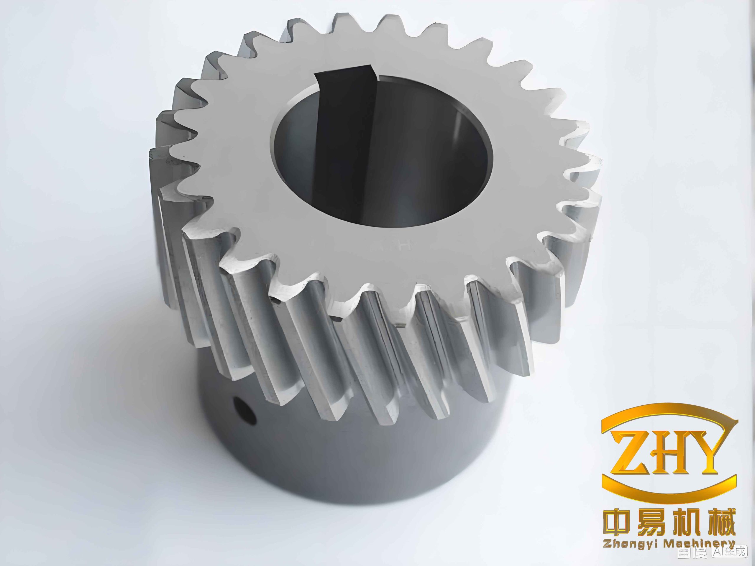
1. Meshing Kinematics and Contact-Line Behavior of Helical Gears
I begin with the meshing process because the dynamic excitation of helical gears is strongly related to the continuous change in contact-line length and the number of simultaneously engaged tooth pairs. For helical gears, the contact line is inclined across the tooth face, and the total contact length varies periodically with the rotation angle. This periodic variation is smoother than that of spur gears, but it still produces internal excitation when the number of meshing tooth pairs changes. I define the transverse contact ratio and the overlap contact ratio as:
$$ \varepsilon_\alpha = \frac{z_1\left(\tan\alpha_{at1}-\tan\alpha_t’\right)+z_2\left(\tan\alpha_{at2}-\tan\alpha_t’\right)}{2\pi} $$
$$ \varepsilon_\beta = \frac{B\sin\beta}{\pi m_n} $$
$$ \varepsilon = \varepsilon_\alpha + \varepsilon_\beta $$
Here, \(z_1\) and \(z_2\) are the tooth numbers of the pinion and gear, \(\alpha_{at1}\) and \(\alpha_{at2}\) are the transverse pressure angles at the addendum circles, \(\alpha_t’\) is the transverse operating pressure angle, \(B\) is the face width, \(\beta\) is the helix angle, and \(m_n\) is the normal module. For helical gears, the total contact ratio is usually greater than that of comparable spur gears, so the average load per tooth pair is lower and the transmission is smoother. However, the instantaneous contact-line length still changes with the meshing position.
I divide one meshing cycle into several phases according to the number of loaded tooth pairs. In the low-contact-ratio and high-contact-ratio cases, the contact-line length of a single tooth pair can be expressed in piecewise form. For \(\varepsilon_\alpha < \varepsilon_\beta\), I write:
$$ L_i(\theta)=
\begin{cases}
0, & \theta_1 \le \theta \le \theta_2 \\
\dfrac{B}{\sin\beta}\dfrac{\theta-\theta_2}{\theta_5-\theta_2}, & \theta_2 \le \theta \le \theta_5 \\
\dfrac{B}{\sin\beta}\dfrac{\theta_7-\theta}{\theta_7-\theta_5}, & \theta_5 \le \theta \le \theta_7
\end{cases}
$$
For \(\varepsilon_\alpha \ge \varepsilon_\beta\), a similar piecewise description holds with the characteristic angles shifted by the overlap contact ratio. The total contact-line length at any instant is:
$$ L(\theta)=\sum_{i=1}^{n}L_i(\theta) $$
The load-sharing coefficient of tooth pair \(i\) is then:
$$ \Lambda_i(\theta)=\frac{L_i(\theta)}{L(\theta)} $$
This relation shows that the load distribution among helical gears is not constant. When the number of meshing pairs changes, the contact-line length and load-sharing coefficient jump or change slope, and these changes act as internal excitations. I summarize the main meshing phases in Table 1.
| Phase | Condition | Number of Tooth Pairs | Dynamic Consequence |
|---|---|---|---|
| Entering mesh | New pair begins contact | Increases by one | Contact-line slope changes; local load decreases |
| Double-to-triple transition | \(\theta=\theta_1,\theta_3,\theta_6\) | 2 to 3 | Load sharing redistributes; mesh stiffness rises |
| Triple-to-double transition | \(\theta=\theta_4,\theta_2\) | 3 to 2 | Load per pair increases; flash temperature rises |
| Recess | Pair leaves contact | Decreases by one | Local sliding speed and flash temperature peak |
The contact-line length is affected by module, tooth-number ratio, pressure angle, and helix angle. I summarize the trends I observe in Table 2.
| Parameter | Variation | Effect on Contact-Line Length | Stability Implication |
|---|---|---|---|
| Module \(m_n\) | Increases | Amplitude \(\Delta L\) increases | Stable double-pair region narrows |
| Tooth-number ratio | Increases | Curve shifts downward; amplitude weakly affected | Load capacity changes but trend remains smooth |
| Pressure angle \(\alpha_n\) | Increases | Double-pair region widens; triple-pair region narrows | Excessive pressure angle lowers contact length |
| Helix angle \(\beta\) | Decreases | Inclination angle increases; curve approaches spur-gear behavior | Tooth impact becomes more severe |
2. Sliding Velocity and Entrainment Velocity in Helical Gears
I next compute the kinematic quantities that control lubrication and friction. At a point \(K\) along the line of action, the radii of curvature of the pinion and gear are:
$$ R_1 = r_1\sin\alpha_n – x_k, \qquad R_2 = r_2\sin\alpha_n + x_k $$
The equivalent radius is:
$$ R = \frac{R_1 R_2}{R_1+R_2} $$
The tangential velocities of the two tooth surfaces are:
$$ u_1 = \omega_1 R_1, \qquad u_2 = \omega_2 R_2 $$
The relative sliding velocity and the entrainment velocity are:
$$ u_s = u_1-u_2 $$
$$ u_e = \frac{u_1+u_2}{2} $$
The slide-to-roll ratio is:
$$ SR = \frac{u_s}{u_e} $$
For helical gears, the sliding velocity changes sign at the pitch point and reaches its largest absolute value near the engage and recess points. The entrainment velocity generally increases from engage to recess. I show representative trends in Table 3.
| Quantity | At Engage | At Pitch Point | At Recess |
|---|---|---|---|
| Relative sliding velocity | Large negative | Zero | Large positive |
| Entrainment velocity | Lower | Intermediate | Higher |
| Slide-to-roll ratio | Large negative | Zero | Large positive |
| Flash temperature risk | High | Low | Highest |
3. Line-Contact Thermal Elastohydrodynamic Model
I treat the meshing tooth pair as a finite line contact between two elastic cylinders. The Hertzian half-width and maximum pressure are:
$$ a = \sqrt{\frac{8wR}{\pi E’}} $$
$$ \frac{1}{E’} = \frac{1}{2}\left(\frac{1-\nu_1^2}{E_1}+\frac{1-\nu_2^2}{E_2}\right) $$
$$ p_H = \frac{2w}{\pi a} $$
The pressure distribution in the Hertzian region is:
$$ p(x)=p_H\sqrt{1-\left(\frac{x}{a}\right)^2}, \qquad -a \le x \le a $$
For the lubricated line contact, I use the Reynolds equation:
$$ \frac{d}{dx}\left(\frac{\rho h^3}{\eta}\frac{dp}{dx}\right)=12u_e\frac{d(\rho h)}{dx} $$
The energy equation for the lubricant film is:
$$ \rho c_p\left(u\frac{\partial T}{\partial x}+w\frac{\partial T}{\partial z}\right)-\beta_T T u\frac{\partial p}{\partial x}=K\frac{\partial^2 T}{\partial z^2}+\eta\left(\frac{\partial u}{\partial z}\right)^2 $$
The film thickness includes the initial central film, the geometric gap, elastic deformation, and thermal deformation:
$$ h(x)=h_0+\frac{x^2}{2R}-\frac{2}{\pi E’}\int_{x_i}^{x_e}p(s)\ln(s-x)^2ds+\delta_T $$
I use a Roelands-type viscosity equation:
$$ \eta = \eta_0 \exp\left\{(\ln\eta_0+9.67)\left[(1+5.1\times10^{-9}p)^Z\left(1+1.1\times10^{-3}(T-T_0)\right)^{-S}-1\right]\right\} $$
The density variation is:
$$ \rho = \rho_0\left[1+\frac{0.6p}{1+1.7p}+D(T-T_0)\right] $$
The load balance is:
$$ w=\int_{x_i}^{x_e}p(x)dx $$
I solve these equations with dimensionless variables and a finite-difference discretization. The dimensionless Reynolds equation is:
$$ \frac{d}{dX}\left(\varepsilon\frac{dP}{dX}\right)=\frac{d(\bar{\rho}H)}{dX} $$
where
$$ \varepsilon=\frac{\bar{\rho}H^3}{\bar{\eta}\lambda}, \qquad \lambda=\frac{12u_e\eta_0R^2}{a^3p_H} $$
The energy equation becomes:
$$ A\bar{\rho}\left(\bar{u}\frac{\partial \bar{T}}{\partial X}\right)+B\bar{\rho}\bar{u}\frac{\partial P}{\partial X}=C\frac{\partial^2 \bar{T}}{\partial Z^2}+D\bar{\eta}\left(\frac{\partial \bar{u}}{\partial Z}\right)^2 $$
I use a multigrid method with Gauss-Seidel iteration and Jacobi dipole iteration. The overall solution procedure is summarized in Table 4.
| Step | Action | Purpose |
|---|---|---|
| 1 | Set initial pressure and temperature fields | Provide starting fields for iteration |
| 2 | Compute film thickness and viscosity | Update lubricant properties |
| 3 | Solve Reynolds equation | Obtain new pressure distribution |
| 4 | Solve energy equation | Obtain temperature distribution |
| 5 | Update viscosity and density | Couple thermal and pressure effects |
| 6 | Check load balance and convergence | Ensure physical consistency |
| 7 | Transfer residuals across multigrid levels | Accelerate convergence |
4. Line-Contact Lubrication Results for Helical Gears
I examine how speed, transmitted power, and lubricant viscosity affect the oil-film pressure, film thickness, and flash temperature of helical gears. As the rotational speed increases, the entrainment velocity increases, the film thickness rises, and the minimum film location moves away from the outlet region. At low speed, the second pressure peak is weak or absent. As speed rises, the second pressure peak appears, grows, and moves upstream. The flash temperature also rises with speed because the frictional heat generation increases. I summarize these trends in Table 5.
| Operating Change | Film Thickness | Second Pressure Peak | Flash Temperature | Lubrication State |
|---|---|---|---|---|
| Speed increases | Increases | Appears and grows | Increases | Stronger EHL film |
| Power increases | Decreases slightly | Decreases | Increases | Higher thermal load |
| Viscosity decreases | Decreases | Decreases and disappears | Increases | Risk of dry contact |
| Load increases | Decreases | Decreases | Increases | Thinner film, higher stress |
Viscosity is highly sensitive to temperature. When the tooth surface temperature increases, the lubricant viscosity first drops sharply and then tends toward a lower plateau. This reduces the load-carrying capacity of the oil film. If the film becomes too thin, asperity contact occurs and the helical gears may experience scuffing, wear, and surface fatigue. I represent the viscosity-temperature relation in a general form as:
$$ \eta(T)=\eta_0\exp\left[-S\ln\left(1+\frac{T-T_0}{T_0-138}\right)\right] $$
For a line-contact case, I write the dimensionless film thickness as:
$$ H(X)=H_0+\frac{X^2}{2}-\frac{1}{2\pi}\int_{X_i}^{X_e}P(X’)\ln(X-X’)^2dX’+\delta_T $$
The load balance in dimensionless form is:
$$ \int_{X_i}^{X_e}P(X)dX=\frac{\pi}{2} $$
5. Point-Contact Thermal Elastohydrodynamic Model at Engage and Recess
Although line contact describes most of the meshing path, the engage and recess points of helical gears often involve point-like contact or edge contact. I therefore build a point-contact thermal elastohydrodynamic model. The Reynolds equation for point contact is:
$$ \frac{\partial}{\partial x}\left(\frac{\rho h^3}{\eta}\frac{\partial p}{\partial x}\right)+\frac{\partial}{\partial y}\left(\frac{\rho h^3}{\eta}\frac{\partial p}{\partial y}\right)=12u_e\frac{\partial(\rho h)}{\partial x} $$
The film thickness is:
$$ h(x,y)=h_0+\frac{x^2}{2R_x}+\frac{y^2}{2R_y}+\frac{2}{\pi E’}\iint_{\Omega}\frac{p(x’,y’)}{\sqrt{(x-x’)^2+(y-y’)^2}}dx’dy’+\delta_T $$
The energy equation in the film is:
$$ \rho c_p\left(u\frac{\partial T}{\partial x}+v\frac{\partial T}{\partial y}\right)-\beta_T T\left(u\frac{\partial p}{\partial x}+v\frac{\partial p}{\partial y}\right)=K\left(\frac{\partial^2 T}{\partial z^2}\right)+\eta\left[\left(\frac{\partial u}{\partial z}\right)^2+\left(\frac{\partial v}{\partial z}\right)^2\right] $$
The load balance is:
$$ F=\iint_{\Omega}p(x,y)dxdy $$
I solve the point-contact equations with a multigrid method. The boundary conditions are zero pressure at the inlet and outlet and zero pressure gradient at the outlet. The numerical procedure uses weighted restriction and interpolation between coarse and fine grids. I summarize the algorithm in Table 6.
| Component | Method | Role |
|---|---|---|
| Pressure equation | Gauss-Seidel iteration | Solves Reynolds equation on each grid |
| Elastic deformation | Jacobi dipole iteration | Computes surface displacement |
| Multigrid cycle | V-cycle | Reduces low- and high-frequency errors |
| Restriction | Weighted restriction operator | Transfers residuals to coarse grids |
| Interpolation | Weighted interpolation operator | Transfers corrections to fine grids |
| Rigid-body correction | Load balance update | Enforces prescribed load |
At the engage point, the equivalent radius is smaller and the contact stress is lower than at the recess point. The oil-film pressure is lower, the film is thicker, and the flash temperature begins to rise. At the recess point, the load per tooth pair is higher, the sliding velocity is larger, and the entrainment velocity is also high. The oil-film pressure becomes columnar, with a sharp increase inside the contact region. The film-thickness distribution is basin-shaped, with a concave central region and minimum film at the contact edge. The flash-temperature distribution follows the pressure distribution and reaches its maximum near the recess point. I compare the point-contact results in Table 7.
| Quantity | Engage Region | Recess Region | Physical Meaning |
|---|---|---|---|
| Maximum oil-film pressure | Lower | Higher | Load concentration near recess |
| Minimum film thickness | Thicker | Thinner | Higher risk of asperity contact |
| Flash temperature | Lower | Higher | Stronger frictional heating |
| Pressure shape | Moderate column | Sharp column | Point-contact pressure concentration |
| Film shape | Basin-shaped | Basin-shaped with deeper edge minimum | Elastic deformation and thermal softening |
The point-contact flash temperature is much higher than the line-contact flash temperature. This is important for helical gears because the engage and recess regions are where scuffing and wear often begin. The combination of high sliding speed, high load, thin film, and high flash temperature can break the lubricant film and cause direct metal-to-metal contact.
6. Dynamic Excitations in Helical Gear Transmission Systems
I now define the main internal excitations that enter the dynamic model. The backlash function is:
$$ f(p)=
\begin{cases}
p-b, & p>b \\
0, & |p|\le b \\
p+b, & p<-b
\end{cases}
$$
In dimensionless form, with \(\lambda=p/b\),
$$ f(\lambda)=
\begin{cases}
\lambda-1, & \lambda>1 \\
0, & |\lambda|\le 1 \\
\lambda+1, & \lambda<-1
\end{cases}
$$
The static transmission error is expanded as a Fourier series:
$$ e(t)=e_0+\sum_{j=1}^{\infty}e_j\cos(j\omega_e t+\phi_j) $$
For most dynamic studies, I retain the first harmonic:
$$ e(t)=e_0+e_1\cos(\omega_e t) $$
The mesh stiffness of a single tooth pair is represented by a Gaussian-like function:
$$ K_i(s)=k_p C_a \exp\left[-\frac{(s-s_p)^2}{2.25\varepsilon_{bt}^2}\right] $$
The total mesh stiffness is:
$$ K(s)=\sum_{i=1}^{n}K_i(s) $$
When flash temperature is included, the oil-film stiffness is computed from the distributed pressure and film thickness:
$$ k_f=\sum_{i=1}^{n}\frac{L\,p(x_i)}{h(x_i)} $$
The time-varying mesh stiffness with flash temperature is:
$$ k_T(t)=k_m(t)+k_f(T) $$
I fit the stiffness curve with a Fourier series:
$$ k(t)=\frac{a_0}{2}+\sum_{n=1}^{N}\left[a_n\cos(n\omega t)+b_n\sin(n\omega t)\right] $$
The friction coefficient is computed from an empirical relation involving lubricant viscosity, surface roughness, equivalent radius, maximum Hertzian pressure, and slide-to-roll ratio:
$$ \mu=\mu_0 e^{b_1}SR^{b_2}P_H^{b_3}S^{b_4}R^{b_5}\eta_0^{b_6} $$
The friction force for tooth pair \(i\) is:
$$ f_i(t)=\mu_i(t)w_i(t)\operatorname{sgn}(u_s) $$
The total friction force is:
$$ F_f(t)=\sum_{i=1}^{n}f_i(t) $$
The friction torque on the pinion and gear is:
$$ T_{fp}(t)=\sum_{i=1}^{n}f_i(t)L_{pi}(t), \qquad T_{fg}(t)=\sum_{i=1}^{n}f_i(t)L_{gi}(t) $$
The friction coefficient is zero at the pitch point because the relative sliding velocity is zero. It reaches extreme values near the engage and recess points. I summarize the friction-related excitations in Table 8.
| Excitation | Origin | Time Variation | Effect on Helical Gears |
|---|---|---|---|
| Backlash | Assembly and thermal expansion | Piecewise nonlinear | Impact, tooth separation, noise |
| Transmission error | Manufacturing and mounting error | Periodic | Parametric excitation |
| Mesh stiffness | Contact-line variation and oil film | Periodic with jumps | Parametric excitation and stability change |
| Friction | Sliding and lubricant state | Sign-changing periodic | Torque fluctuation and thermal load |
| Flash temperature | Frictional heat | Strongly position-dependent | Viscosity drop, film thinning, stiffness reduction |
7. Nonlinear Dynamic Model of Helical Gears with Flash Temperature
I use a lumped-mass model for the helical gear pair. The model includes transverse motions of the pinion and gear in the \(y\) and \(z\) directions, as well as torsional motion. The relative displacement along the line of action is:
$$ p=(y_p-y_g)\sin\beta-(z_p-z_g)\cos\beta-(r_{pb}\theta_p-r_{gb}\theta_g)-e(t) $$
The dynamic mesh force is:
$$ F_n=k_T f(p)+c_m\dot{p} $$
The components along \(y\) and \(z\) are:
$$ F_y=F_n\cos\beta, \qquad F_z=F_n\sin\beta $$
The equations of motion without flash temperature are:
$$ m_p\ddot{y}_p+c_{py}\dot{y}_p+k_{py}y_p=-F_y $$
$$ m_g\ddot{y}_g+c_{gy}\dot{y}_g+k_{gy}y_g=F_y $$
$$ m_p\ddot{z}_p+c_{pz}\dot{z}_p+k_{pz}z_p=-F_z $$
$$ m_g\ddot{z}_g+c_{gz}\dot{z}_g+k_{gz}z_g=F_z $$
$$ I_p\ddot{\theta}_p+r_{pb}F_n=T_p $$
$$ I_g\ddot{\theta}_g-r_{gb}F_n=-T_g $$
When flash temperature is included, friction torques are added:
$$ I_p\ddot{\theta}_p+r_{pb}F_n=T_p-T_{fp} $$
$$ I_g\ddot{\theta}_g-r_{gb}F_n=-T_g+T_{fg} $$
The transverse equations become:
$$ m_p\ddot{y}_p+c_{py}\dot{y}_p+k_{py}y_p=-F_y+F_{fy} $$
$$ m_g\ddot{y}_g+c_{gy}\dot{y}_g+k_{gy}y_g=F_y-F_{fy} $$
$$ m_p\ddot{z}_p+c_{pz}\dot{z}_p+k_{pz}z_p=-F_z+F_{fz} $$
$$ m_g\ddot{z}_g+c_{gz}\dot{z}_g+k_{gz}z_g=F_z+F_{fz} $$
By combining the torsional equations, I obtain the equivalent dynamic equation:
$$ m_e\ddot{p}+c_m\dot{p}+k_T f(p)=F_{pm}+F_e+F_\mu $$
where the equivalent mass is:
$$ m_e=\frac{I_p I_g}{I_p r_{gb}^2+I_g r_{pb}^2} $$
The internal excitation is:
$$ F_e=m_e e_1\omega_e^2\cos(\omega_e t) $$
The external excitation is:
$$ F_{pm}=m_e\left(\frac{r_{pb}T_p}{I_p}+\frac{r_{gb}T_g}{I_g}\right) $$
The friction excitation is:
$$ F_\mu=m_e\left(\frac{r_{pb}T_{fp}}{I_p}-\frac{r_{gb}T_{fg}}{I_g}\right) $$
I introduce dimensionless time and frequency:
$$ \tau=\omega_n t, \qquad \omega_n=\sqrt{\frac{k_m}{m_e}}, \qquad \Omega=\frac{\omega_e}{\omega_n} $$
The dimensionless displacement is:
$$ \lambda=\frac{p}{b} $$
The dimensionless dynamic equation is:
$$ \lambda”+2\zeta\lambda’+\kappa_T f(\lambda)=f_a\cos(\Omega\tau)+f_m+F_\mu $$
where
$$ \zeta=\frac{c_m}{2m_e\omega_n}, \qquad \kappa_T=\frac{k_T}{m_e\omega_n^2} $$
I integrate the resulting state equations with a fourth-fifth order Runge-Kutta method. The state vector is:
$$ \mathbf{x}=\left[y_1,\dot{y}_1,y_2,\dot{y}_2,z_1,\dot{z}_1,z_2,\dot{z}_2,\lambda,\dot{\lambda}\right]^T $$
The state equations have the form:
$$ \dot{\mathbf{x}}=\mathbf{F}(\mathbf{x},\tau,\Omega) $$
8. Bifurcation Behavior Without Flash Temperature
I first analyze the helical gear system without flash temperature. The bifurcation parameter is the dimensionless meshing frequency \(\Omega\). In the low-frequency range, the system undergoes single-period motion, period-two motion, quasi-periodic motion, period-three motion, and chaotic motion. A jump appears in the bifurcation diagram, and the Poincaré section changes from one point to a closed curve or a fractal set. I summarize the low-frequency behavior in Table 9.
| Frequency Range | Observed Motion | Poincaré Section | Dynamic Feature |
|---|---|---|---|
| \(\Omega<0.5667\) | Single period | One point | Stable periodic response |
| \(\Omega=0.5667\) | Quasi-periodic transition | Closed curve | Chaotic attractor begins to form |
| \(\Omega\in(0.5922,0.5948)\) | Period six | Six points | Brief periodic window |
| \(\Omega=0.6196\) | Return to single period | One point | Attractor collapses |
| \(\Omega=0.6446\) | Period three and chaos | Three points and fractal | Route to chaos |
In the mid-frequency range, the system exhibits saddle-node bifurcation, period doubling, and period-doubling degradation. A single-double saddle-node bifurcation occurs near \(\Omega=1.1810\). A single-period to period-three saddle-node bifurcation occurs near \(\Omega=1.5720\). After a short chaotic region, the system returns to single-period motion through a series of period-doubling degradations.
In the high-frequency range, the system shows alternating chaotic and periodic windows. Quasi-periodic motion appears near \(\Omega=1.7220\), and chaotic attractors split as \(\Omega\) increases. Period doubling occurs near \(\Omega=2.4914\), followed by period-four motion, then degradation back to period-two and finally single-period motion. I summarize the high-frequency behavior in Table 10.
| Frequency Range | Motion Type | Key Feature |
|---|---|---|
| \(\Omega\in(1.60,1.71)\) | Chaos and single period alternate | Multiple windows |
| \(\Omega=1.7220\) | Quasi-periodic | Chaotic attractor splitting |
| \(\Omega=1.7457\) | Chaotic | Fractal Poincaré section |
| \(\Omega=1.9992\) | Single period | Chaos disappears |
| \(\Omega=2.4914\) | Period two | Period-doubling bifurcation |
| \(\Omega=2.4958\) | Period four | Second period-doubling |
| \(\Omega=2.6050\) | Period-two degradation | Reverse period doubling |
| \(\Omega=2.6680\) | Single period | Stable periodic motion |
9. Bifurcation Behavior With Flash Temperature
I then include flash temperature through the thermal EHL oil-film stiffness and the friction excitation. The global bifurcation diagram changes significantly. The chaotic region becomes smaller, and the system tends to return to periodic motion earlier. The jump point moves to a lower frequency, and the post-jump motion becomes period-two rather than remaining single-period. Quasi-periodic motion appears earlier and exits earlier. The chaotic attractor undergoes distortion and splitting, and periodic windows appear inside the quasi-periodic region. I summarize the main differences in Table 11.
| Frequency Range | Without Flash Temperature | With Flash Temperature | Physical Reason |
|---|---|---|---|
| Low frequency | Jump, quasi-period, period-six, chaos | Earlier jump, period-two, period-five, chaos reduced | Oil film and friction dissipate energy |
| Mid frequency | Saddle-node, period doubling, degradation | Similar route but smoother return to period-one | Thermal effect weakens stiffness jumps |
| High frequency | Alternating chaos and period windows | More complex windows; chaotic region reduced overall | Thermal softening and film thinning compete |
In the low-frequency range, the mesh damping increases and the time-varying mesh stiffness decreases when flash temperature is considered. The lubricant film and friction dissipate part of the vibration energy. As a result, the original quasi-periodic motion, saddle-node bifurcation, and chaotic motion occur earlier, and some chaotic or quasi-periodic motions degrade into periodic motion. The system is more likely to stabilize. In the mid-frequency range, the route into chaos is not fundamentally changed, but the return to single-period motion is smoother and lacks the abrupt jump seen without flash temperature. In the high-frequency range, the influence of flash temperature is more complicated. There are many interwoven windows of periodic, quasi-periodic, and chaotic motion. Boundary crises, attractor distortion, and attractor splitting appear. The system has difficulty escaping chaos after entering it, and some chaotic regions are prolonged. However, the overall chaotic area is still smaller than in the isothermal case.
I express the dimensionless mesh stiffness with flash temperature as:
$$ \kappa_T(\tau)=\kappa_m(\tau)+\kappa_f(\tau) $$
where \(\kappa_f\) is the oil-film stiffness contribution. The friction excitation is:
$$ F_\mu(\tau)=F_{\mu 0}+\sum_{n=1}^{N}\left[a_{\mu n}\cos(n\Omega\tau)+b_{\mu n}\sin(n\Omega\tau)\right] $$
The friction torque fitting coefficients are obtained from the point-contact and line-contact thermal EHL results. I use an eight-order Fourier series for the stiffness and a fifth-order Fourier series for the friction torque to avoid discontinuities in the differential equation. The fitted expressions are smooth enough for time integration.
10. Influence of Flash Temperature on Stability of Helical Gears
I can now state the main dynamic consequences. For helical gears operating at low frequency, flash temperature tends to stabilize the system. The oil film acts as a compliant layer, and the friction forces dissipate energy. The chaotic region shrinks, and periodic windows become wider. For helical gears operating at middle frequency, flash temperature has a relatively small effect on the route to chaos, but it smooths the transition back to periodic motion. For helical gears operating at high frequency, flash temperature produces competing effects. On one hand, the oil film reduces stiffness and adds damping. On the other hand, high flash temperature reduces viscosity and film thickness, which can increase asperity contact and friction. This competition creates complex bifurcation windows and intermittent chaos.
The most important design implication is that flash temperature cannot be ignored in the dynamic analysis of high-speed helical gears. It changes the mesh stiffness, friction excitation, and oil-film state. The thermal effect is not a small perturbation. It modifies the bifurcation topology, shifts the critical frequencies, and changes the size and location of chaotic regions. I summarize the design implications in Table 12.
| Operating Regime | Dominant Effect | Stability Trend | Design Recommendation |
|---|---|---|---|
| Low frequency | Oil-film damping and friction dissipation | Stabilizing | Use thermal EHL in stability prediction |
| Mid frequency | Smooth stiffness reduction | Weakly stabilizing | Control transmission error and backlash |
| High frequency | Competition between film damping and thermal thinning | Complex, partially destabilizing | Improve cooling and lubricant supply |
11. Numerical Implementation and Verification Strategy
I implement the thermal EHL solver with dimensionless variables. The line-contact solver uses a one-dimensional grid along the rolling direction. The point-contact solver uses a two-dimensional grid over the elliptical contact region. The dynamic solver uses a fourth-fifth order Runge-Kutta method with adaptive time stepping. The Poincaré section is sampled once per meshing period. I check convergence by refining the grid and reducing the time step. The load balance is enforced at each iteration. The viscosity and density are updated from the current pressure and temperature. The elastic deformation is computed by a multilevel integration of the pressure field.
The dimensionless groups that control the problem are:
$$ U=\frac{u_e\eta_0}{E’R}, \qquad W=\frac{w}{E’R}, \qquad G=\alpha E’ $$
For point contact, I also use the ellipticity ratio:
$$ k=\frac{b}{a} $$
The thermal loading parameter is:
$$ L_T=\frac{\beta_T u_e^2\eta_0}{K} $$
These groups show that speed, load, material properties, and lubricant rheology are coupled. A change in flash temperature changes the viscosity and film thickness, which in turn changes the friction coefficient and mesh stiffness. This two-way coupling is the core of the present dynamic characterization.
12. Conclusions
I have developed a coupled thermal elastohydrodynamic and nonlinear dynamic model for helical gear transmission systems with flash temperature. The model starts from the meshing kinematics of helical gears and includes contact-line length, load sharing, sliding velocity, entrainment velocity, line-contact thermal EHL, point-contact thermal EHL, backlash, transmission error, mesh damping, friction, and time-varying mesh stiffness. The main conclusions are as follows.
First, the contact-line length of helical gears varies continuously with the meshing position. The variation is smoother than that of spur gears, but the change in the number of meshing tooth pairs still creates internal excitation. Module, pressure angle, and helix angle strongly affect the contact-line curve. Larger module and excessive pressure angle reduce the stable double-pair region, while smaller helix angle makes the helical gears behave more like spur gears and increases tooth impact.
Second, the lubricant viscosity is highly sensitive to flash temperature. As temperature rises, viscosity drops sharply and then tends toward a lower plateau. The oil-film thickness decreases, the second pressure peak weakens and moves toward the outlet, and the risk of asperity contact increases. Higher speed increases film thickness and flash temperature. Higher transmitted power increases flash temperature and reduces the second pressure peak. The load and sliding speed jointly determine the maximum pressure and minimum film thickness.
Third, point contact at the engage and recess regions is more severe than line contact. The oil-film pressure is columnar, the film thickness is basin-shaped, and the minimum film appears at the contact edge. The flash temperature follows the pressure field and reaches its maximum near the recess point. The engage and recess regions are therefore critical for scuffing, wear, and surface fatigue in helical gears.
Fourth, flash temperature reduces the time-varying mesh stiffness but does not change its overall trend. It also changes the friction coefficient and friction torque. The friction coefficient is zero at the pitch point and reaches extreme values near the engage and recess points. The friction torque is periodic and sign-changing, and it must be included as a dynamic excitation.
Fifth, the nonlinear dynamic response of helical gears is strongly affected by flash temperature. In the low-frequency range, the system is stabilized. The quasi-periodic, saddle-node, and chaotic regions appear earlier, and some chaotic and quasi-periodic motions degrade into periodic motion. In the mid-frequency range, the route into chaos is similar, but the return to periodic motion is smoother. In the high-frequency range, the response becomes more complex. Period, quasi-period, and chaos are interwoven, and the system has difficulty escaping chaos after entering it. However, the overall chaotic region is still smaller when flash temperature is included.
Finally, I conclude that flash temperature must be treated as a coupled dynamic variable in the design and analysis of high-speed helical gears. It is not merely a thermal side effect. It changes the oil-film state, the mesh stiffness, the friction excitation, and the bifurcation topology. For reliable operation of helical gears, the designer should consider thermal EHL effects, cooling capacity, lubricant viscosity, surface roughness, and dynamic stability together rather than separately.