
This article presents a comprehensive investigation into the dynamic modeling and vibration response analysis of spur gear transmission systems with localized defects. The study covers the establishment of a multi-degree-of-freedom dynamic model for a compound fault spur gear transmission, the introduction of gyroscopic motion of the transmission shaft to couple the gear pair and supporting bearings, and the inclusion of bearing housing clearance effects. The paper also proposes an advanced fault diagnosis method based on multi-sensor information fusion and a two-stream convolutional neural network (TSCNN). Analytical results are validated through experiments. The findings reveal that variable operating conditions, gear-bearing coupling, and bearing clearance significantly influence the vibration characteristics of the spur gear system, providing a theoretical basis for precise condition monitoring and fault diagnosis of spur gear transmissions.
1. Introduction
Spur gear transmission systems are widely employed in modern mechanical industry owing to their stable instantaneous transmission ratio, high transmission efficiency, and long service life. However, harsh working environments, lubrication failures, fatigue wear, and assembly errors often induce localized defects on gear teeth and bearing components, threatening the safe and reliable operation of the equipment. Condition monitoring based on vibration signals is essential to ensure operational reliability. The vibration characteristics of a spur gear system are complex, especially when defects coexist on multiple components, making accurate state identification challenging. Therefore, establishing realistic dynamic models that capture the interactions between gears and bearings is of great significance.
This work focuses on the dynamic modeling and vibration response analysis of spur gear transmission systems with localized defects. The main contributions include: (1) establishing a compound fault spur gear transmission dynamic model with variable operating conditions; (2) incorporating the gyroscopic motion of the transmission shaft to establish gear-bearing coupling relationships; (3) introducing bearing outer ring and housing clearance into the coupled dynamic model; and (4) proposing a novel diagnostic model named OWF-TSCNN for effective fault type and severity identification. Throughout the paper, the term spur gear is used to emphasize the gear type under study.
2. Dynamic Modeling of a Compound Fault Spur Gear Transmission
A 36-degree-of-freedom (DOF) dynamic model of a spur gear transmission system is established using Lagrange’s equation. The model includes the input shaft, the output shaft, four supporting bearings, the driving spur gear, the driven spur gear, and the load. In this model, both gear tooth spalling and localized bearing defects are considered. The governing equations are presented below.
The input shaft torsional equation is:
$$
I_{f1}\ddot{\theta}_{f1} + c_{f1}(\dot{\theta}_{f1}-\dot{\theta}_{pin}) + k_{f1}(\theta_{f1}-\theta_{pin}) = T_1
\tag{1}
$$
For bearing 1, the five equations describing the inner race, outer race, and resonator displacements are:
$$
\begin{cases}
m_{s1}\ddot{x}_{s1} + c_{s1}(\dot{x}_{s1}-\dot{x}_{pin}) + k_{s1}(x_{s1}-x_{pin}) + f_{x1} = 0,\\[2mm]
m_{s1}\ddot{y}_{s1} + c_{s1}(\dot{y}_{s1}-\dot{y}_{pin}) + k_{s1}(y_{s1}-y_{pin}) + f_{y1} = 0,\\[2mm]
m_{p1}\ddot{x}_{p1} + c_{p1}\dot{x}_{p1} + k_{p1}x_{p1} – f_{x1} = 0,\\[2mm]
m_{p1}\ddot{y}_{p1} + (c_{p1}+c_{r1})\dot{y}_{p1} + (k_{p1}+k_{r1})y_{p1} – k_{r1}y_{r1} – c_{r1}\dot{y}_{r1} – f_{y1} = 0,\\[2mm]
m_{r1}\ddot{y}_{r1} + c_{r1}(\dot{y}_{r1}-\dot{y}_{p1}) + k_{r1}(y_{r1}-y_{p1}) = 0.
\end{cases}
\tag{2}
$$
The contact forces in the x and y directions are calculated from the Hertzian contact theory as:
$$
\begin{cases}
f_{x1} = k_{re1}\sum_{i=1}^{n_b} \gamma_i \delta_i^{n} \cos\theta_i,\\[2mm]
f_{y1} = k_{re1}\sum_{i=1}^{n_b} \gamma_i \delta_i^{n} \sin\theta_i,
\end{cases}
\tag{3}
$$
where \(k_{re1}\) is the equivalent contact stiffness, \(n_b\) is the number of rollers, \(n=1.5\) for rolling bearings, \(\gamma_i\) is a switching function:
$$
\gamma_i =
\begin{cases}
1, & \delta_i > 0,\\
0, & \text{otherwise},
\end{cases}
\tag{4}
$$
and \(\theta_i\) is the angular position of the \(i\)-th roller:
$$
\theta_i = \frac{2\pi (i-1)}{n_b} + \left(1-\frac{d_b}{d_m}\right)\frac{\omega_s}{2} t + \theta_0,
\tag{5}
$$
where \(d_b\) is the roller diameter, \(d_m\) is the pitch diameter, \(\omega_s\) is the inner race speed, \(\theta_0\) is the initial cage phase, and \(t\) is time. The contact deformation \(\delta_i\) is:
$$
\delta_i = (x_s – x_p)\cos\theta_i + (y_s – y_p)\sin\theta_i – c_o – h_d,
\tag{6}
$$
where \(c_o\) is the radial clearance and \(h_d\) is the additional displacement caused by a localized bearing defect. For a healthy bearing, \(h_d=0\). For an outer race defect:
$$
h_d =
\begin{cases}
L_{or}, & \theta_{oc} < \theta_i < \theta_{oc} + \frac{L_{ol}}{d_o},\\[2mm]
0, & \text{otherwise},
\end{cases}
\tag{7}
$$
and for an inner race defect:
$$
h_d =
\begin{cases}
L_{ir}, & \theta_{ic} < (\omega_i t – \theta_i) < \theta_{ic} + \frac{L_{il}}{d_i},\\[2mm]
0, & \text{otherwise}.
\end{cases}
\tag{8}
$$
Here \(L_{or}, L_{ol}\) are the depth and length of the outer race defect, \(\theta_{oc}\) is its initial phase, \(d_o\) is the outer race diameter, \(L_{ir}, L_{il}\) are the depth and length of the inner race defect, \(\theta_{ic}\) is the inner race defect initial phase, and \(\omega_i\) is the inner race angular speed.
3. Time-Varying Mesh Stiffness of Spur Gear with Spalling Defect
For a spur gear pair with a rectangular spalling defect, the mesh stiffness is reduced because the cross-sectional area \(A_x\) and the area moment of inertia \(I_x\) change. According to the potential energy method, the bending stiffness \(k_b\), shear stiffness \(k_s\), and radial compressive stiffness \(k_a\) can be derived. The detailed expressions are:
$$
\frac{1}{k_b} = \int_{-\alpha_1}^{-\alpha_x}
\frac{3\{1+\cos\alpha_1[(\alpha_2-\alpha)\sin\alpha-\cos\alpha]\}^2(\alpha_2-\alpha)\cos\alpha}
{2EL[\sin\alpha + (\alpha_2-\alpha)\cos\alpha]^3} \, d\alpha
$$
$$
+ \int_{-\alpha_x}^{\alpha_s}
\frac{12\{1+\cos\alpha_1[(\alpha_2-\alpha)\sin\alpha-\cos\alpha]\}^2(\alpha_2-\alpha)\cos\alpha}
{E\{8L[\sin\alpha + (\alpha_2-\alpha)\cos\alpha]^3 – (h_s R_{b1})^3 a_s\}} \, d\alpha
$$
$$
+ \int_{\alpha_s}^{\alpha_2}
\frac{3\{1+\cos\alpha_1[(\alpha_2-\alpha)\sin\alpha-\cos\alpha]\}^2(\alpha_2-\alpha)\cos\alpha}
{2EL[\sin\alpha + (\alpha_2-\alpha)\cos\alpha]^3} \, d\alpha,
\tag{9}
$$
where \(a_s\), \(b_s\), and \(h_s\) are the length, width, and depth of the spalling defect. Similarly, the shear stiffness is:
$$
\frac{1}{k_s} = \int_{-\alpha_1}^{-\alpha_x}
\frac{1.2(1+\nu)(\alpha_2-\alpha)\cos\alpha \cos^2\alpha_1}
{EL[\sin\alpha + (\alpha_2-\alpha)\cos\alpha]} \, d\alpha
$$
$$
+ \int_{-\alpha_x}^{\alpha_s}
\frac{2.4(1+\nu)(\alpha_2-\alpha)\cos\alpha \cos^2\alpha_1}
{E\{2L[\sin\alpha + (\alpha_2-\alpha)\cos\alpha] – (h_s/R_{b1})a_s\}} \, d\alpha
$$
$$
+ \int_{\alpha_s}^{\alpha_2}
\frac{1.2(1+\nu)(\alpha_2-\alpha)\cos\alpha \cos^2\alpha_1}
{EL[\sin\alpha + (\alpha_2-\alpha)\cos\alpha]} \, d\alpha,
\tag{10}
$$
and the radial compressive stiffness is:
$$
\frac{1}{k_a} = \int_{-\alpha_1}^{-\alpha_x}
\frac{(\alpha_2-\alpha)\cos\alpha \sin^2\alpha_1}
{2EL[\sin\alpha + (\alpha_2-\alpha)\cos\alpha]} \, d\alpha
$$
$$
+ \int_{-\alpha_x}^{\alpha_s}
\frac{(\alpha_2-\alpha)\cos\alpha \sin^2\alpha_1}
{E\{2L[\sin\alpha + (\alpha_2-\alpha)\cos\alpha] – (h_s/R_{b1})a_s\}} \, d\alpha
$$
$$
+ \int_{\alpha_s}^{\alpha_2}
\frac{(\alpha_2-\alpha)\cos\alpha \sin^2\alpha_1}
{2EL[\sin\alpha + (\alpha_2-\alpha)\cos\alpha]} \, d\alpha.
\tag{11}
$$
The total mesh stiffness of a spur gear pair is then obtained by summing the individual compliances:
$$
\frac{1}{k_t} =
\begin{cases}
\displaystyle \sum_{i=1}^{2}\left(\frac{1}{k_{b1,i}}+\frac{1}{k_{s1,i}}+\frac{1}{k_{a1,i}}+\frac{1}{k_{h,i}}+\frac{1}{k_{f1,i}}+\frac{1}{k_{b2,i}}+\frac{1}{k_{s2,i}}+\frac{1}{k_{a2,i}}+\frac{1}{k_{f2,i}}\right), & \text{double-tooth contact},\\[6mm]
\displaystyle \frac{1}{k_{b1}}+\frac{1}{k_{s1}}+\frac{1}{k_{a1}}+\frac{1}{k_{h}}+\frac{1}{k_{f1}}+\frac{1}{k_{b2}}+\frac{1}{k_{s2}}+\frac{1}{k_{a2}}+\frac{1}{k_{h}}+\frac{1}{k_{f2}}, & \text{single-tooth contact}.
\end{cases}
\tag{12}
$$
Table 1 summarizes the main parameters used in the spur gear transmission dynamic model.
| Parameter | Value |
|---|---|
| Mass of driving spur gear, \(m_{pin}\) | 0.96 kg |
| Mass of driven spur gear, \(m_{ge}\) | 2.88 kg |
| Moment of inertia of driving spur gear, \(I_{pin}\) | 4.365e-4 kg·m² |
| Moment of inertia of driven spur gear, \(I_{ge}\) | 8.362e-4 kg·m² |
| Input shaft inertia, \(I_{f1}\) | 0.0021 kg·m² |
| Output shaft inertia, \(I_{f2}\) | 0.0105 kg·m² |
| Shaft torsional stiffness, \(k_{f1}, k_{f2}\) | 4.4e4 N·m/rad |
| Shaft torsional damping, \(c_{f1}, c_{f2}\) | 5.0e5 N·m·s/rad |
| Bearing support stiffness, \(k_{sj}, k_{pj}, k_{rj}\) | 6.56e7 N/m |
| Bearing support damping, \(c_{sj}, c_{pj}, c_{rj}\) | 1.8e5 N·s/m |
| Mean transmission error, \(e_o\) | 2e-5 m |
| Transmission error amplitude, \(e_m\) | 3e-5 m |
| Parameter | Driving gear | Driven gear |
|---|---|---|
| Module \(m\) (mm) | 2.5 | 2.5 |
| Number of teeth \(z\) | 23 | 81 |
| Pressure angle \(\alpha\) (deg) | 20 | 20 |
| Face width \(L\) (mm) | 26 | 26 |
| Elastic modulus \(E\) (GPa) | 206 | 206 |
| Poisson ratio \(\nu\) | 0.3 | 0.3 |
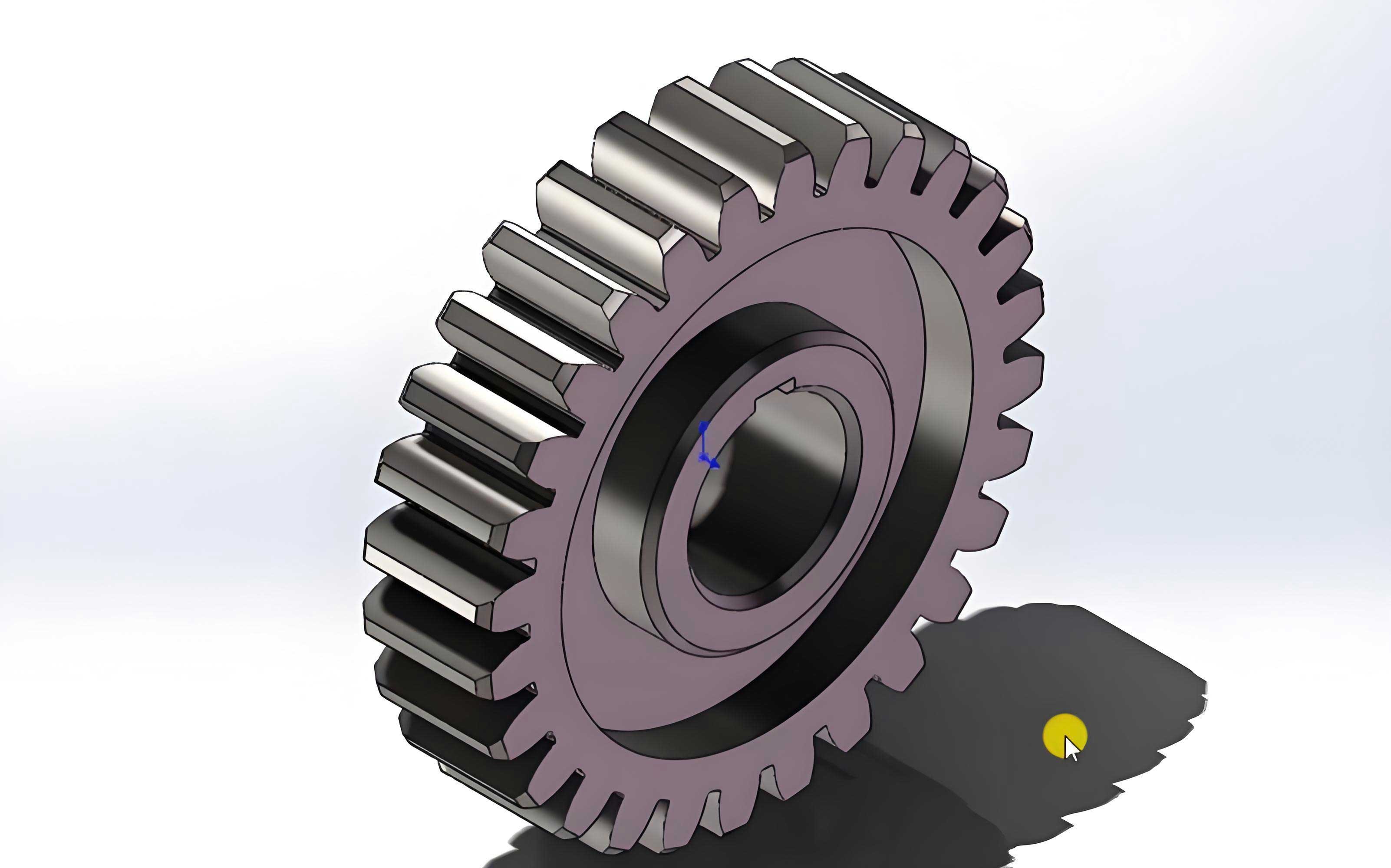
A picture of a typical spur gear set used in transmission systems is shown below.
4. Dynamic Response under Variable Operating Conditions
Variable speed and variable load conditions introduce non-stationarity into the vibration signals of a faulted spur gear transmission. The short-time Fourier transform (STFT) is employed to process the non-stationary signals. Simulations are carried out with a compound fault consisting of a spalling defect on the driving spur gear and a pitting defect on bearing 1 outer race or inner race.
4.1 Variable Speed Condition
When the motor speed increases from 1800 rpm at a rate of 600 rpm/s under a constant load of 30 N·m, the vibration response of bearing 1 resonator is obtained. The time–frequency spectrum indicates that the spur gear meshing frequency \(f_m\) and its harmonics, such as \(f_m-3f_{r1}\) and \(f_m-4f_{r1}\), appear. For the bearing outer race defect, the fault frequency \(f_{o1}\) is observed. With increasing speed, the magnitudes of all fault frequencies increase.
For a bearing inner race defect, the fault frequencies \(f_{i1}\), \(2f_{i1}\), and \(3f_{i1}\) are identified along with their modulations with the shaft rotational frequency \(f_{r1}\). The pseudo-order spectra show fixed order lines: the gear order \(O_m=23\), the outer race order \(O_o=2.57\), and the inner race order \(O_i=4.43\). The amplitudes of these order lines increase with speed. Table 3 shows the characteristic fault frequencies for the spur gear and bearing.
| Component / Defect | Characteristic Frequency (Hz) |
|---|---|
| Spur gear meshing | \(f_m = z_1 f_{r1}\) |
| Bearing outer race defect | \(f_{o} = \frac{n_b}{2} f_{r1} \left(1 – \frac{d_b}{d_m}\right)\) |
| Bearing inner race defect | \(f_{i} = \frac{n_b}{2} f_{r1} \left(1 + \frac{d_b}{d_m}\right)\) |
| Roller defect | \(f_{r} = \frac{f_{r1}}{2} \frac{d_m}{d_b} \left(1 – \frac{d_b^2}{d_m^2}\right)\) |
4.2 Variable Load Condition
When the motor speed is constant at 1800 rpm and the load torque increases from 15 N·m to 30 N·m, the vibration response shows that the fault frequencies remain unchanged in frequency but their amplitudes increase steadily. This is observed for both outer race and inner race bearing defects combined with spur gear spalling. The amplitude growth is attributed to the higher contact force acting on the defect region.
4.3 Speed and Load Fluctuations
When the motor speed fluctuates about a target value, e.g., \(f = f’ + A\sin(2\pi t + \phi_1)\), the fault frequencies and their amplitudes fluctuate with the same trend. Similarly, when the load torque fluctuates, the frequency amplitudes follow the load fluctuation. These results demonstrate that variable operating conditions must be accounted for in condition monitoring of spur gear systems.
5. Coupling Relationship between Spur Gear and Bearing
In a physical spur gear transmission, vibrations of the bearing inner races cause the transmission shaft to perform gyroscopic motion. This motion induces a time-varying center distance error and a misalignment angle in the spur gear pair. These geometric variations modulate the mesh stiffness. The coupling relationship is established by expressing the actual center distance \(a’\) and the misalignment angle \(\theta\) in terms of the bearing inner race displacements:
$$
\theta = \arccos\frac{\sqrt{(x_{s2}-x_{s1})^2 + (y_{s2}-y_{s1})^2}}
{\sqrt{(x_{s2}-x_{s1})^2 + (y_{s2}-y_{s1})^2 + L^2}},
\tag{13}
$$
$$
a’ = \sqrt{\left[a-\frac{1}{2}(x_{s1}+x_{s2})\right]^2 + \frac{1}{4}(y_{s1}+y_{s2})^2},
\tag{14}
$$
where \(L\) is the shaft length and \(a\) is the nominal center distance. The misalignment causes the load to be distributed non-uniformly along the tooth width, resulting in an additional torsional stiffness \(k_\tau\). The stiffness expressions are modified by multiplying \(\cos^2\theta\) terms and adding \(k_\tau\) to the total compliance. The gear mesh stiffness in the coupled model becomes:
$$
\frac{1}{k_t} =
\begin{cases}
\displaystyle \sum_{i=1}^{2}\left(\frac{1}{k_{b1,i}}+\frac{1}{k_{s1,i}}+\frac{1}{k_{a1,i}}+\frac{1}{k_{h,i}}+\frac{1}{k_{f1,i}}+\frac{1}{k_{b2,i}}+\frac{1}{k_{s2,i}}+\frac{1}{k_{a2,i}}+\frac{1}{k_{f2,i}}+\frac{1}{k_{\tau1,i}}+\frac{1}{k_{\tau2,i}}\right), & \text{double}\\[6mm]
\displaystyle \frac{1}{k_{b1}}+\frac{1}{k_{s1}}+\frac{1}{k_{a1}}+\frac{1}{k_{h}}+\frac{1}{k_{f1}}+\frac{1}{k_{b2}}+\frac{1}{k_{s2}}+\frac{1}{k_{a2}}+\frac{1}{k_{h}}+\frac{1}{k_{f2}}+\frac{1}{k_{\tau1}}+\frac{1}{k_{\tau2}}, & \text{single}.
\end{cases}
\tag{15}
$$
Simulation results for a healthy spur gear transmission show that the center distance error and misalignment angle vary periodically with the meshing period. When a spalling defect exists on the driving spur gear, the center distance and misalignment angle exhibit abrupt changes whenever the defect enters the meshing zone, causing a further reduction in mesh stiffness. Similarly, when the bearing inner race has a local defect, the induced displacement causes impulsive changes in the center distance and misalignment angle, thereby affecting the meshing stiffness of the spur gear pair. This coupling explains why the spectrum of a single bearing defect also contains spur gear meshing frequencies and why a single spur gear defect excites bearing characteristic frequencies.
Table 4 summarizes the fault-induced spectral components observed in the coupled spur gear transmission system.
| Fault condition | Observed frequencies in the bearing housing response |
|---|---|
| Healthy spur gear system | \(f_m\), \(2f_m\), \(3f_m\), small sidebands \(f_m \pm f_{r1}\) |
| Spur gear spalling only | \(f_m\), \(2f_m\), \(3f_m\), \(f_m \pm f_{r1}\), \(f_m \pm 2f_{r1}\), plus bearing outer race frequency \(f_{o1}\) |
| Bearing inner race defect only | \(nf_m\), \(f_{i1}\), \(2f_{i1}\), \(f_{i1}\pm f_{r1}\), \(2f_{i1}\pm f_{r1}\), plus sidebands \(f_m\pm f_{r1}\) and \(f_m \pm 2f_{r1}\) |
| Compound spalling + inner race defect | Harmonics of \(f_m\), \(f_m\pm f_{r1}\), \(f_{i1}\), \(f_{i1}\pm f_{r1}\), \(2f_{i1}\pm f_{r1}\), with increased amplitudes |
6. Effects of Bearing Housing Clearance on the Spur Gear Transmission
In practical operations, temperature rise and assembly wear may create a clearance between the outer ring and the bearing housing. This clearance causes severe gyroscopic motion of the shaft and introduces nonlinear impact and friction forces between the outer ring and the housing. The impact force \(P_N\) and friction force \(P_T\) are calculated using Hertz theory and Coulomb friction law:
$$
P_N = \left[\frac{(r-\delta)L^2}{0.8 \times 3.83\times10^{-5}}\right]^{10/9} + c_N \dot{r},
\tag{16}
$$
$$
P_T = f P_N \, \text{sign}(v_T),
\tag{17}
$$
where \(r = \sqrt{x_{p1}^2 + y_{p1}^2}\) is the radial displacement of the outer ring center, \(\delta\) is the clearance, \(L\) is the contact length, \(c_N\) is the damping coefficient, \(f\) is the friction coefficient, and \(v_T\) is the tangential velocity. When the clearance is present, the support stiffness and damping of the outer ring are set to zero:
$$
k_{px1} = k_{py1} = 0,\qquad c_{px1} = c_{py1} = 0.
\tag{18}
$$
The numerical results reveal the following:
- The time-domain response of the spur gear system becomes amplitude-modulated by the bearing outer race fault frequency \(f_{o1}\). The modulation effect intensifies as the clearance increases.
- The frequency spectrum contains superharmonic components of both the bearing fault frequency (e.g., \(10f_{o1}, 11f_{o1}, 12f_{o1}, 18f_{o1}\)) and the spur gear meshing frequency (e.g., \(4f_m, 5f_m, 6f_m, 7f_m\)). Higher-order superharmonics are excited when the clearance is larger.
- The shaft orbit becomes irregular and chaotic due to the combined effects of gear meshing impacts and housing clearance impacts. With larger clearance, the number of vibration decay cycles increases, producing more peaks in the polar plot, which corresponds to the appearance of superharmonic resonances.
- Increasing the input speed increases the overall vibration amplitude, but suppresses the superharmonic response. The spur gear system then vibrates predominantly at its fundamental frequencies, indicating that high speed conditions can weaken the harmful superharmonic resonances caused by clearance.
Table 5 compares the dynamic behavior for different clearance values.
| Clearance (mm) | Time domain | Frequency domain | Shaft orbit |
|---|---|---|---|
| 0 (healthy) | Stable, periodic, no obvious modulation | Fundamental meshing frequencies and few sidebands | Near-elliptical, limited region |
| 0.01 | Slight modulation by \(f_{o1}\) | Mild superharmonics, e.g., \(10f_{o1}, 4f_m\) | Elliptical with slightly increased spreads |
| 0.03 | Obvious modulation, larger peaks | Higher order superharmonics, \(11f_{o1}, 5f_m\), sidebands | Irregular orbit with multiple loops |
| 0.05 | Severe amplitude modulation, many shocks | High-order superharmonics, \(18f_{o1}, 7f_m\), dense sidebands | Chaotic and wide-spread orbit |
7. Experimental Verification and Fault Diagnosis of Spur Gear Transmission
To verify the theoretical models and to develop a robust diagnostic strategy, experiments are performed on a spur gear transmission test rig. The test rig includes a motor, a gearbox with a spur gear pair, four cylindrical roller bearings, and a magnetic powder brake. Defects are introduced on the driving spur gear (rectangular spalling of different sizes) and on bearing components (outer race crack, roller crack, and cage fracture). Four acceleration sensors are installed on the bearing housings to measure vertical vibration signals. Table 6 lists the experimental groups.
| Experiment | Spur gear (driving) | Bearing outer race | Roller | Cage | Label |
|---|---|---|---|---|---|
| 1 | Healthy (T) | T | T | T | 1 |
| 2 | F (1mm×7mm) | F (0.2×0.2 mm) | T | T | 2 |
| 3 | F (1mm×7mm) | T | F (0.2×0.2 mm) | T | 3 |
| 4 | F (1mm×7mm) | T | T | F (0.2 mm) | 4 |
| 5 | F (2mm×13mm) | F (0.5×0.5 mm) | T | T | 5 |
| 6 | F (2mm×13mm) | T | F (0.5×0.5 mm) | T | 6 |
| 7 | F (2mm×13mm) | T | T | F (0.5 mm) | 7 |
| 8 | F (4mm×17mm) | F (0.8×0.8 mm) | T | T | 8 |
| 9 | F (4mm×17mm) | T | F (0.8×0.8 mm) | T | 9 |
| 10 | F (4mm×17mm) | T | T | F (0.8 mm) | 10 |
7.1 Multi-Sensor Information Fusion
The vibration signals from four sensors are fused at the data level using the optimal weighting factor (OWF) method. For \(n\) sensors, the fused signal is:
$$
X = \sum_{i=1}^{n} W_i x_i, \qquad \sum_{i=1}^{n} W_i = 1,
\tag{19}
$$
where the optimal weights minimizing the total mean square error are:
$$
W_i = \frac{1}{\sigma_i^2 \sum_{j=1}^{n} (1/\sigma_j^2)},
\tag{20}
$$
and the minimum mean square error is:
$$
\sigma_{\min}^2 = \frac{1}{\sum_{i=1}^{n} (1/\sigma_i^2)}.
\tag{21}
$$
Prior to fusion, each signal is denoised using the dual-tree complex wavelet transform (DT-CWT), which provides approximate shift invariance and better direction selectivity than the standard discrete wavelet transform.
7.2 Two-Stream CNN Model
The proposed diagnostic model OWF-TSCNN combines a one-dimensional CNN (1D-CNN) and a two-dimensional CNN (2D-CNN). The 1D-CNN takes the FFT spectrum of the fused signal as input, while the 2D-CNN takes the wavelet time-frequency image as input. The architecture parameters are given in Tables 7 and 8.
| Layer | Kernel/Stride | Number of kernels | Output size | Activation |
|---|---|---|---|---|
| Input | – | – | 1×433 | – |
| Conv1D-1 | 1×5, 1 | 6 | 6@1×429 | ReLU |
| Pooling1D-1 | 1×3, 3 | 6 | 6@1×143 | – |
| BN-1D-1 | – | 6 | 6@1×143 | – |
| Conv1D-2 | 1×3, 1 | 16 | 16@1×141 | ReLU |
| Pooling1D-2 | 1×3, 3 | 16 | 16@1×47 | – |
| BN-1D-2 | – | 16 | 16@1×47 | – |
| Flatten-1D | – | – | 1×752 | – |
| Layer | Kernel/Stride | Number of kernels | Output size | Activation |
|---|---|---|---|---|
| Input | – | – | 64×64×3 | – |
| Conv2D-1 | 5×5, 1 | 6 | 6@60×60 | ReLU |
| Pooling2D-1 | 2×2, 2 | 6 | 6@30×30 | – |
| BN-2D-1 | – | 6 | 6@30×30 | – |
| Conv2D-2 | 5×5, 1 | 16 | 16@26×26 | ReLU |
| Pooling2D-2 | 2×2, 2 | 16 | 16@13×13 | – |
| BN-2D-2 | – | 16 | 16@13×13 | – |
| Flatten-2D | – | – | 1×1024 | – |
After flattening, the features from both streams are concatenated in a fusion layer:
$$
\mathbf{f} = [\mathbf{f}_{1D}; \mathbf{f}_{2D}],
\tag{22}
$$
where \(\mathbf{f}_{1D}\) has size 1×752 and \(\mathbf{f}_{2D}\) has size 1×1024, resulting in a concatenated feature vector of length 1776. This vector passes through a fully connected layer with 120 neurons and then a second fully connected layer with 84 neurons, both using ReLU activation. Finally, a support vector machine (SVM) classifier with a Gaussian radial basis function kernel is used to categorize the features into 10 fault classes:
$$
f(\mathbf{x}) = \text{sgn}\left[\sum_{n=1}^{e} y_n \lambda_n K(\mathbf{x}, \mathbf{x}_n) + b\right],
\tag{23}
$$
with
$$
K(\mathbf{x}, \mathbf{x}_n) = \exp\left(-\frac{\|\mathbf{x}-\mathbf{x}_n\|^2}{2\sigma^2}\right).
\tag{24}
$$
7.3 Diagnostic Performance
The diagnostic performance of OWF-TSCNN is compared with that of OWF-1DCNN (using only the FFT spectrum input to a 1D-CNN), OWF-2DCNN (using only the wavelet time-frequency image input to a 2D-CNN), and VCR-TSCNN (using variance contribution rate fusion together with the two-stream CNN). Table 9 presents the comparative results after convergence.
| Model | Training accuracy (%) | Test accuracy (%) | Loss entropy | Overfitting ratio | Training time (s) |
|---|---|---|---|---|---|
| OWF-1DCNN | 99.65 | 96.83 | 0.0014 | 1.0801 | 218 |
| OWF-2DCNN | 99.86 | 97.41 | 0.00043 | 1.0453 | 234 |
| VCR-TSCNN | 100 | 99.58 | 0.00015 | 1.0022 | 276 |
| OWF-TSCNN | 100 | 99.93 | 0.00016 | 1.0020 | 268 |
The OWF-TSCNN model achieves the highest test accuracy (99.93%) with relatively low training time compared with VCR-TSCNN. Although the two-stream model increases the training time by 14.5%–26.6% compared to single-stream models, the improvements in accuracy, loss entropy, and overfitting ratio are significant. The confusion matrix for OWF-TSCNN shows 100% classification accuracy for all ten fault types, including different severities. This demonstrates that the combination of multi-sensor OWF fusion and dual-domain feature extraction (time–frequency image and FFT spectrum) greatly enhances the feature extraction capability and generalization ability of the fault diagnosis system for spur gear transmissions.
8. Conclusion
This article has systematically studied the dynamic modeling and vibration response analysis of faulted spur gear transmission systems. The main conclusions are summarized as follows:
- A 36-DOF dynamic model of a compound fault spur gear transmission was established. Under variable speed and load conditions, the non-stationary response processed by STFT reveals that accelerating speed increases both fault frequencies and their amplitudes, while increasing load keeps frequencies unchanged but increases amplitudes. Speed and load fluctuations produce corresponding fluctuations in fault frequency amplitudes.
- The coupling relationship between the spur gear pair and the supporting bearings was modeled through the gyroscopic motion of the transmission shaft. It was found that bearing inner race displacements cause time-varying center distance error and misalignment angle, which reduce the mesh stiffness of the spur gear pair. Local defects on either the spur gear or the bearing induce abrupt changes in these geometric parameters, further deteriorating the mesh stiffness. The spectrum of a single fault contains characteristic frequencies of both the spur gear and the bearing, confirming the coupling effects.
- The presence of bearing housing clearance significantly affects the vibration response. It intensifies the amplitude modulation of the bearing outer race fault frequency, excites superharmonic responses of both the spur gear and bearing, and increases the complexity of the shaft orbit. Increasing the input speed suppresses superharmonic responses, making the system vibrate predominantly at fundamental frequencies.
- An OWF-TSCNN diagnostic model was proposed for spur gear transmission fault diagnosis. By fusing multi-sensor signals with the optimal weighting factor method and utilizing both FFT spectra and wavelet time-frequency images, the model achieves superior classification accuracy, lower loss entropy, and better generalization compared with single-stream CNN models. Experiments verified the correctness of the dynamic models and the effectiveness of the diagnostic approach.
The results presented in this article provide valuable theoretical insights and practical guidance for condition monitoring and fault diagnosis of spur gear transmission systems.