
As a core component in robotic systems, the rotary vector reducer plays a critical role in ensuring precise motion control. Its transmission accuracy directly impacts the performance, reliability, and efficiency of robots. However, due to the complex structure of the rotary vector reducer, factors such as manufacturing errors, assembly tolerances, and meshing gaps can significantly degrade transmission precision. To address this, I have developed an equivalent error modeling approach combined with parameter optimization techniques to enhance the design accuracy of rotary vector reducers. This article presents a comprehensive analysis, including model formulation, parameter identification, optimization using an improved genetic algorithm, and experimental validation.
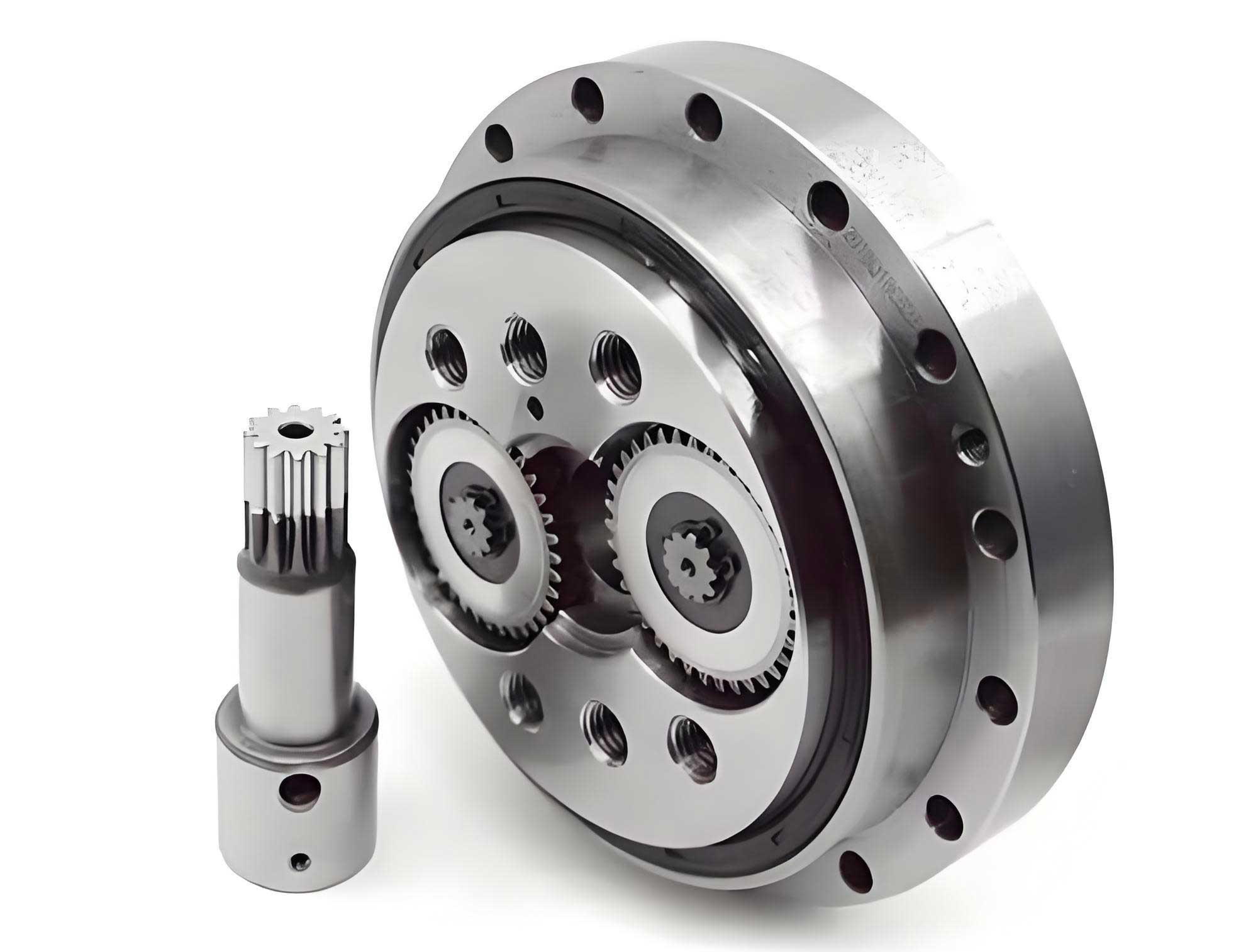
The rotary vector reducer, often abbreviated as RV reducer, is a two-stage reduction device. The first stage involves a planetary gear system, while the second stage utilizes a cycloidal-pin gear mechanism. This configuration provides high reduction ratios, compactness, and low backlash, making it ideal for robotic joints. However, the transmission error, defined as the deviation between the theoretical and actual output angles, arises from various sources. These include stiffness variations in bearings and gear contacts, as well as geometric errors. To systematically analyze these effects, I adopt an equivalent error model that simplifies the complex interactions into spring-mass systems, representing stiffness and error components.
The equivalent error model transforms the rotary vector reducer into a set of rigid bodies connected by springs, where each spring corresponds to a specific stiffness parameter or error source. This approach allows for the derivation of dynamic equations that describe the force-displacement relationships within the reducer. Key parameters in the model include stiffness values for gear meshing, bearing supports, and other contact interfaces. By solving these equations, I can predict the transmission error under various operating conditions.
In the equivalent error model, the rotary vector reducer is represented with coordinates and variables as summarized in the following table:
| Parameter | Description |
|---|---|
| \(O_j\) | Center of mass of the \(j\)-th cycloidal gear near the input side |
| \((X, Y)\) | Coordinate system with origin at the center of the sun gear |
| \((\eta_j, \xi_j)\) | Coordinate system for the \(j\)-th cycloidal gear with \(\eta_j\) as the eccentric direction |
| \(\phi_i\) | Relative position of the \(i\)-th planet gear’s center of mass |
| \(\psi_j\) | Relative position of the \(j\)-th cycloidal gear’s center of mass |
| \(\theta_s\) | Theoretical rotation angle of the input shaft |
| \(\theta_{oj}\) | Rotation angle due to self-rotation of the \(j\)-th cycloidal gear |
| \(\theta_{doj}\) | Rotation angle due to revolution of the \(j\)-th cycloidal gear |
| \(\theta_{ca}\) | Simulated output angle of the rotary vector reducer |
The dynamic equations for each component are derived based on force equilibrium. For the sun gear, the equations are:
$$
\sum_{i=1}^{2} R_{spi} S_{spi} \cos(\gamma_i) + R_s (X_s – a_{SX}) = 0,
$$
$$
\sum_{i=1}^{2} R_{spi} S_{spi} \sin(\gamma_i) + R_s (Y_s – a_{SY}) = 0,
$$
where \(R_{spi}\) is the meshing stiffness between the sun gear and the \(i\)-th planet gear, \(S_{spi}\) is the equivalent displacement along the meshing line, \(\gamma_i\) is the angle of the meshing line relative to the X-axis, \(R_s\) is the support stiffness of the gear shaft, \(X_s\) and \(Y_s\) are displacements, and \(a_{SX}\) and \(a_{SY}\) are assembly errors.
For the planet gears, the dynamic equations are:
$$
S_{spi} R_{spi} \cos \gamma_i – \sum_{j=1}^{2} R_{pd} S_{djix} – R_b S_{cix} = 0,
$$
$$
S_{spi} R_{spi} \sin \gamma_i – \sum_{j=1}^{2} R_{pd} S_{djiy} – R_b S_{ciy} = 0,
$$
$$
S_{spi} R_{spi} a_{sp} + e \sum_{j=1}^{2} (R_{pd} S_{djix} \sin B_j + R_{pd} S_{djiy} \cos B_j) = 0,
$$
where \(R_{pd}\) is the stiffness of cylindrical roller bearings, \(S_{djix}\) and \(S_{djiy}\) are equivalent displacements, \(R_b\) is the stiffness of tapered roller bearings, \(S_{cix}\) and \(S_{ciy}\) are displacements at the crank bearing, \(a_{sp}\) is the center distance, \(e\) is the eccentricity, and \(B_j\) is the theoretical self-rotation angle of the \(j\)-th cycloidal gear.
For the cycloidal gears, the equations are:
$$
\sum_{i=1}^{2} (R_{pd} S_{djix} \sin B_j + R_{pd} S_{djiy} \cos B_j) + \sum_{k=1}^{m} R_{djk} S_{djk} \sin \alpha_{jk} = 0,
$$
$$
\sum_{i=1}^{2} (R_{pd} S_{djiy} \sin B_j – R_{pd} S_{djix} \cos B_j) + \sum_{k=1}^{m} R_{djk} S_{djk} \cos \alpha_{jk} = 0,
$$
$$
\sum_{i=1}^{2} a_{sp} (R_{pd} S_{djiy} \cos P_i – R_{pd} S_{djix} \sin P_i) + r_d \sum_{k=1}^{m} R_{djk} S_{djk} \sin \alpha_{jk} = 0,
$$
where \(R_{djk}\) is the meshing stiffness between the \(j\)-th cycloidal gear and the \(k\)-th pin gear, \(S_{djk}\) is the equivalent displacement, \(\alpha_{jk}\) is the angle of the meshing line, \(P_i\) is the theoretical rotation angle of the \(i\)-th crank, and \(r_d\) is the pitch circle radius of the cycloidal gear.
For the planetary carrier, the dynamic equations are:
$$
\sum_{i=1}^{2} R_b S_{cix} – R_{ca} (X_{ca} – a_{cx}) = 0,
$$
$$
\sum_{i=1}^{2} R_b S_{ciy} – R_{ca} (Y_{ca} – a_{cy}) = 0,
$$
$$
a_{sp} \sum_{i=1}^{2} (R_b S_{cix} \sin P_i – R_b S_{ciy} \cos P_i) = T_{out},
$$
where \(R_{ca}\) is the stiffness of angular contact bearings, \(X_{ca}\) and \(Y_{ca}\) are displacements, \(a_{cx}\) and \(a_{cy}\) are assembly errors, and \(T_{out}\) is the output torque.
These equations are combined into a matrix form:
$$
\mathbf{R} \mathbf{Y} = \mathbf{P},
$$
where \(\mathbf{R}\) is a \(17 \times 17\) stiffness matrix, \(\mathbf{P}\) is a \(17 \times 1\) force vector, and \(\mathbf{Y}\) is a vector of displacement variables. The output angle from the equivalent model is denoted as \(\hat{\theta}_{ca}\), and the theoretical output angle is \(\theta_c\). The transmission error is then calculated as \(\Delta \theta = \theta_{ca} – \theta_c\) for actual values, and \(\Delta \hat{\theta} = \hat{\theta}_{ca} – \theta_c\) for simulated values.
In the rotary vector reducer, several stiffness parameters influence the transmission error. Key parameters include \(R_{spi}\) (sun-planet meshing stiffness), \(R_s\) (shaft support stiffness), \(R_{djk}\) (cycloidal-pin meshing stiffness), \(R_{ca}\) (angular contact bearing stiffness), \(R_b\) (tapered roller bearing stiffness), and \(R_{pd}\) (cylindrical roller bearing stiffness). However, due to the high reduction ratio, the effects of \(R_{spi}\) and \(R_s\) are minimized after reduction. Additionally, the symmetry of cycloidal gears cancels out the influence of \(R_{djk}\). Therefore, the primary parameters for optimization are \(R_{ca}\), \(R_b\), and \(R_{pd}\). These stiffness values can be estimated using empirical formulas:
$$
R_{ca} = \frac{E_g n_3 r_g^{0.5}}{3(1 – \mu^2)},
$$
$$
R_b = \frac{\pi l_2 E n_2}{8(1 – \mu^2) \sin(80\pi/180)},
$$
$$
R_{pd} = \frac{\pi l_1 E n_1}{8(1 – \mu^2)},
$$
where \(\mu\) is Poisson’s ratio, \(E\) is the elastic modulus of roller materials, \(l_1\) and \(n_1\) are the contact length and number of rollers in cylindrical bearings, \(l_2\) and \(n_2\) are for tapered bearings, \(E_g\) is the elastic modulus of the raceway material, \(n_3\) is the number of balls in angular contact bearings, and \(r_g\) is the pin diameter. These formulas provide initial estimates, but manufacturing variations necessitate optimization for accurate modeling of the rotary vector reducer.
To optimize the stiffness parameters, I formulate a least squares problem. The objective is to minimize the difference between the simulated transmission error peaks (\(\hat{u}_i\)) and the actual measured peaks (\(u_i\)). The optimization model is:
$$
\min \frac{1}{2} \sum_{i=1}^{N} (\hat{u}_i – u_i)^2,
$$
subject to constraints on \(R_{ca}\), \(R_b\), and \(R_{pd}\) based on empirical bounds. This optimization enhances the accuracy of the equivalent error model for the rotary vector reducer.
I employ an improved genetic algorithm to solve this optimization problem. Genetic algorithms are evolutionary search techniques inspired by natural selection, involving initialization, fitness evaluation, selection, crossover, and mutation. However, standard genetic algorithms can suffer from premature convergence and high computational cost. My improved version incorporates the following enhancements:
- Diversity Maintenance: During initialization and iteration, I remove duplicate individuals to prevent population homogeneity. If the number of unique individuals falls below a threshold, new individuals are introduced to maintain diversity.
- Elitism with Immigration: I implement a 20%淘汰 rate (淘汰率, elimination rate) to discard low-fitness individuals, reducing computational waste. This is similar to an immigration operator that replaces weak solutions.
- Dynamic Mutation: The mutation probability is adjusted dynamically. When the population becomes too similar, the mutation rate is increased to introduce new genetic material, accelerating the search for optimal solutions.
The algorithm parameters are set as follows: population size of 100, generations of 100, crossover probability of 0.8, initial mutation probability of 0.2, and elimination probability of 0.2. The fitness function is defined as the inverse of the variance between simulated and actual error peaks:
$$
V = \frac{1}{N} \sum_{i=1}^{N} (\delta_i – \hat{\delta}_i)^2,
$$
$$
\text{Fitness} = \frac{1}{V},
$$
where \(\delta_i\) and \(\hat{\delta}_i\) are the peak-to-peak values of actual and simulated transmission errors, respectively. Binary encoding with a length of 45 bits is used for the parameters.
The optimization process for the rotary vector reducer is illustrated in the flowchart below, though not explicitly shown in text, it involves iterative steps of selection, crossover, mutation, and fitness evaluation until convergence.
To validate the approach, I conduct experiments using a rotary vector reducer test platform. The platform consists of a drive motor, input and output circular gratings for angle measurement, and a load motor. The actual transmission error is calculated by comparing the theoretical output angle (derived from input measurements) with the actual output angle. I use an RV-20E type rotary vector reducer as the test subject, with specifications including a two-stage transmission: first stage with 20 sun gear teeth and 26 planet gear teeth (module 1.5 mm, pressure angle 20°), and second stage with 40 pin teeth and 39 cycloidal gear teeth (pin distribution circle radius 52 mm, eccentricity 0.9 mm).
The improved genetic algorithm is compared with a basic genetic algorithm. In multiple trials, the basic algorithm often exhibits premature convergence, while the improved version consistently converges within 20 generations without premature stagnation. The following table summarizes the optimized stiffness parameters and the corresponding \(V\) index from 10 experimental runs:
| Run | \(R_{ca}\) (×10¹⁰) | \(R_{b}\) (×10¹⁰) | \(R_{pd}\) (×10¹⁰) | \(V\) |
|---|---|---|---|---|
| 1 | 7.933 | 1.786 | 1.101 | 6.553 |
| 2 | 8.017 | 1.799 | 1.100 | 6.574 |
| 3 | 7.933 | 1.799 | 1.101 | 6.553 |
| 4 | 7.899 | 1.803 | 1.101 | 6.553 |
| 5 | 8.038 | 1.793 | 1.100 | 6.574 |
| 6 | 7.989 | 1.790 | 1.101 | 6.574 |
| 7 | 7.929 | 1.788 | 1.101 | 6.553 |
| 8 | 8.033 | 1.782 | 1.101 | 6.553 |
| 9 | 7.933 | 1.786 | 1.101 | 6.553 |
| 10 | 7.996 | 1.789 | 1.100 | 6.574 |
The average values of the optimized parameters and the \(V\) index are compared with pre-optimization estimates:
| Parameter | Range (×10¹⁰) | Pre-optimization Average (×10¹⁰) | Post-optimization Average (×10¹⁰) | Improvement Rate (%) |
|---|---|---|---|---|
| \(R_{ca}\) | [7.4, 8.0] | 7.850 | 7.970 | – |
| \(R_{b}\) | [1.4, 1.8] | 1.640 | 1.792 | – |
| \(R_{pd}\) | [0.8, 1.3] | 1.090 | 1.101 | – |
| \(V\) | – | 8.065 | 6.564 | 18.62 |
The transmission error results for 10 sets of data are shown below, comparing actual errors, theoretical errors from the equivalent model with optimized parameters, and the difference between theoretical and actual errors:
| Data Set | Actual Error Peak (arcsec) | Theoretical Error Peak (arcsec) | Difference Pre-optimization (arcsec) | Difference Post-optimization (arcsec) | Improvement Rate (%) |
|---|---|---|---|---|---|
| 1 | 93.92 | 95.42 | 1.50 | 1.39 | 7.33 |
| 2 | 95.25 | 98.82 | 3.57 | 3.19 | 10.64 |
| 3 | 101.82 | 104.76 | 2.94 | 2.64 | 10.20 |
| 4 | 104.14 | 107.83 | 3.69 | 3.22 | 12.73 |
| 5 | 110.15 | 112.76 | 2.61 | 2.39 | 8.43 |
| 6 | 112.71 | 115.25 | 2.54 | 2.33 | 8.27 |
| 7 | 116.86 | 119.95 | 3.09 | 2.80 | 9.46 |
| 8 | 121.74 | 123.66 | 1.92 | 1.70 | 11.46 |
| 9 | 125.21 | 127.78 | 2.57 | 2.35 | 8.54 |
| 10 | 128.25 | 130.76 | 2.51 | 2.16 | 13.93 |
The results demonstrate that the optimized equivalent error model reduces the average difference between theoretical and actual transmission errors by 10.09%, indicating a significant improvement in design accuracy for the rotary vector reducer. This enhancement is crucial for applications requiring high precision, such as industrial robots and aerospace systems.
In conclusion, the equivalent error modeling approach, combined with parameter optimization using an improved genetic algorithm, provides an effective method for enhancing the transmission accuracy of rotary vector reducers. By focusing on key stiffness parameters and employing advanced optimization techniques, I have achieved a substantial reduction in error predictions. This methodology offers valuable insights for the design and optimization of high-precision rotary vector reducers, contributing to improved performance in robotic and mechanical systems. Future work may involve extending the model to include thermal effects or dynamic loading conditions for further refinement.
The rotary vector reducer, as a critical component, benefits from such detailed analysis, ensuring reliability and efficiency in demanding applications. The repeated emphasis on rotary vector reducer throughout this article underscores its importance in precision engineering. Through continuous innovation in modeling and optimization, the performance boundaries of rotary vector reducers can be pushed further, enabling advancements in automation and technology.