
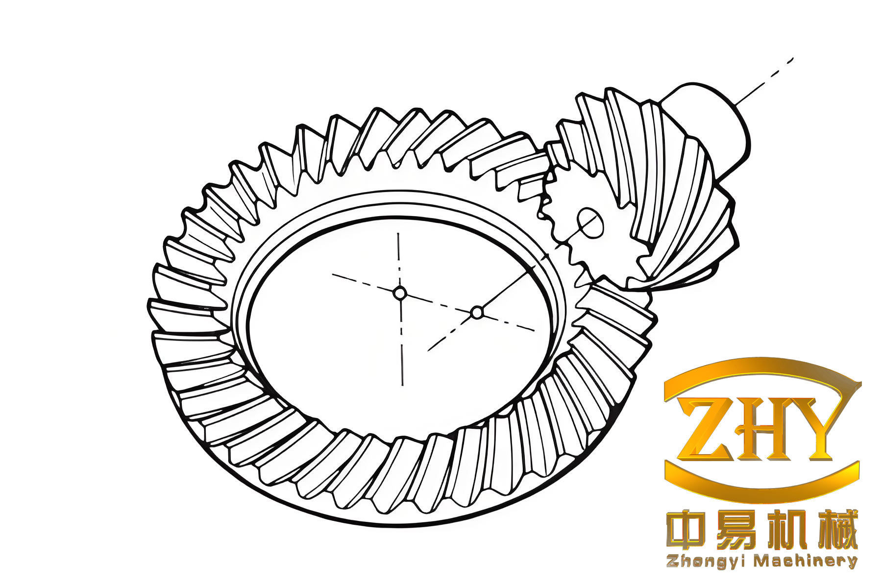
I have dedicated my research to the meshing characteristics of face-hobbed hypoid bevel gears because these gears are widely used in automotive axles, aerospace transmissions, and industrial drive systems. Their advantages include a high contact ratio, strong tolerance to misalignment, smooth transmission, and suitability for large crossed shaft angles with offset axes. In the automotive industry especially, hypoid bevel gears dominate rear axle and four-wheel-drive applications. However, the tooth surface of a face-hobbed hypoid bevel gear is generated by a complex continuous indexing process. A cutter head rotates about its own axis while orbiting about the machine cradle axis, creating an extended epicycloid. The resulting tooth surface is a non-developable ruled surface, which makes mathematical modeling, tooth surface design, and contact pattern control extremely difficult. Unlike face-milled hypoid bevel gears, face-hobbed hypoid bevel gears cannot be ground after heat treatment; only lapping is possible, and lapping only slightly polishes the surface. Consequently, tool errors, machine setting deviations, heat treatment distortions, and assembly misalignments directly affect the final tooth geometry and mesh behavior. In this work, I establish a precise mathematical model, investigate the influence of tool errors and misalignments on mesh characteristics, and verify the model through cutting, measurement, and rolling tests.
1. Geometric Modeling of Face-Hobbed Hypoid Bevel Gears
The face-hobbing process for hypoid bevel gears can be described as a continuous indexing operation. The cutter head contains several groups of blades, and each group has at least one inner blade and one outer blade. The inner blade cuts the convex side, while the outer blade cuts the concave side. As the cutter head rotates, the workpiece also rotates at a predetermined ratio. When the cutter head passes one blade group, the workpiece rotates exactly one tooth pitch. Thus, both sides of a tooth slot are machined simultaneously. The generating surface is the trace of the cutting edges in the machine coordinate system. For the gear member, the process is usually formate (no generation), while for the pinion member, the process is generated (the cradle rolls). This method is known as the tilted half-generating method, or HFT.
I model the cutter head based on the neutral data (ND) normal reference. The cutting edge consists of a main cutting edge and a tip arc. The main cutting edge generates the working tooth flank, and the tip arc generates the root fillet. The main cutting edge can be straight, circular, or polynomial. In my study, I use a circular main cutting edge. The blade is defined on the rake face, and then transformed to the ND plane by considering the rake angle, regrind angle, and cutting side relief angle. The coordinate systems are defined as follows: $$ S_t $$ is fixed to the blade on the rake face; $$ S_{ND} $$ is the neutral data coordinate system; $$ S_c $$ is the cutter head coordinate system; $$ S_m $$ is the machine coordinate system; and $$ S_w $$ is the workpiece coordinate system. The transformation from the blade to the workpiece can be written as a chain of homogeneous matrices.
For the main cutting edge, the position vector in $$ S_t $$ is:
$$ \mathbf{r}_{t}(u) = \begin{bmatrix} R_s \sin\left(\frac{u}{R_s}\right) \\ R_s \left(1 – \cos\left(\frac{u}{R_s}\right)\right) \\ 0 \end{bmatrix} $$
where $$ R_s $$ is the radius of the circular main cutting edge and $$ u $$ is the arc length parameter measured from the reference point. For the tip arc, the position vector is:
$$ \mathbf{r}_{f}(\theta) = \begin{bmatrix} R_f \cos\theta + x_M \\ R_f \sin\theta + y_M \\ 0 \end{bmatrix} $$
where $$ R_f $$ is the tip radius, $$ \theta $$ is the angular parameter, and $$ (x_M, y_M) $$ is the center of the tip arc relative to the reference point. The transformation from $$ S_t $$ to $$ S_{ND} $$ involves rotations about the rake angle $$ \gamma $$, the regrind angle $$ \varepsilon $$, and the cutting side relief angle $$ \alpha_s $$. These rotations can be expressed as:
$$ \mathbf{M}_{ND,t} = \mathbf{R}_x(\alpha_s) \mathbf{R}_y(\varepsilon) \mathbf{R}_z(\gamma) $$
Then, the blade is mounted on the cutter head. The transformation from $$ S_{ND} $$ to the cutter head coordinate system $$ S_c $$ includes the blade offset angle and the radial setting. The cutter head rotates about its own axis, and the machine cradle rotates about the cradle axis. The complete transformation from the cutter head to the workpiece is:
$$ \mathbf{M}_{w,t} = \mathbf{M}_{w,m} \mathbf{M}_{m,c} \mathbf{M}_{c,ND} \mathbf{M}_{ND,t} $$
The machine settings include the radial setting $$ SR $$, the swivel angle $$ j $$, the tilt angle $$ i $$, the initial cradle angle $$ q $$, the vertical offset $$ E $$, the sliding base $$ B $$, the horizontal setting $$ A $$, the machine root angle $$ \gamma_m $$, and the roll ratio $$ i_{gp} $$. For the generated pinion, the tooth surface is the envelope of the family of cutter surfaces. The meshing equation is:
$$ \mathbf{n} \cdot \mathbf{v}^{(12)} = 0 $$
where $$ \mathbf{n} $$ is the unit normal to the cutter surface and $$ \mathbf{v}^{(12)} $$ is the relative velocity between the cutter and the workpiece. Solving this equation together with the cutter surface equation gives the generated tooth surface. For the formate gear, the tooth surface is simply the trace of the cutter surface at the final cradle position.
I implement the above equations in MATLAB to calculate the tooth surface point sets for both pinion and gear. Then I import these point sets into a three-dimensional CAD environment to build the solid models. The modeling workflow is as follows: first, calculate the cutting edge points; second, transform them to the workpiece coordinate system; third, create the tooth slot by sweeping the cutter surface; fourth, perform a Boolean subtraction from the blank; and fifth, assemble the pinion and gear according to the mounting distances. The gear and cutter parameters are listed in Table 1, and the machine settings are listed in Table 2.
| Parameter | Pinion concave | Pinion convex | Gear concave | Gear convex |
|---|---|---|---|---|
| Number of teeth | 11 | 11 | 47 | 47 |
| Hand of spiral | Left | Left | Right | Right |
| Offset distance (mm) | 38.1 | 38.1 | 38.1 | 38.1 |
| Shaft angle (deg) | 90 | 90 | 90 | 90 |
| Modification coefficient | 0.65 | 0.65 | -0.65 | -0.65 |
| Reference point radius (mm) | 76 | 76 | 76 | 76 |
| Cutting edge radius (mm) | 1093.65 | 1062.73 | 1360.74 | 1276.45 |
| Profile pressure angle (deg) | 22.3059 | 20.1933 | 18.9931 | 23.5060 |
| Regrind angle (deg) | 4.3674 | 4.7856 | 5.0309 | 4.1101 |
| Cutting side relief angle (deg) | 13.3885 | 12.6729 | 13.3823 | 12.6781 |
| Rake angle (deg) | 9.5870 | 10.3059 | 12.6781 | 9.6107 |
| Machine parameter | Symbol | Pinion | Gear |
|---|---|---|---|
| Tilt angle (deg) | i | 3.3325 | 0 |
| Swivel angle (deg) | j | 146.9405 | 0 |
| Radial setting (mm) | SR | 121.9391 | 122.009 |
| Initial cradle angle (deg) | q | 52.6673 | -29.7048 |
| Vertical offset (mm) | E | 39.8352 | 0 |
| Sliding base (mm) | B | -12.2486 | 0 |
| Horizontal setting (mm) | A | 3.1158 | 13.9199 |
| Machine root angle (deg) | γ | 23.4453 | 64.7995 |
| Roll ratio | igp | 4.722168 | 0 |
After building the solid models, I check the assembly for interference. The pinion and gear mesh correctly at both the toe and heel ends, which preliminarily validates the mathematical model and the modeling workflow.
2. Tool Errors and Their Influence on Tooth Surface Geometry
In actual manufacturing, tool errors inevitably occur due to regrinding, manufacturing tolerances, and installation deviations. These errors directly affect the tooth surface geometry and, consequently, the meshing characteristics of hypoid bevel gears. I define five tool error parameters: the spheric radius error $$ \Delta R_s $$, the reference point pressure angle error $$ \Delta \alpha_0 $$, the rake angle error $$ \Delta \gamma $$, the regrind angle error $$ \Delta \varepsilon $$, and the cutting side relief angle error $$ \Delta \alpha_s $$. The tooth surface deviation is defined as positive when the error surface is outside the standard surface, and negative when it is inside. I analyze the influence of each error on the pinion concave surface while keeping the convex surface as the standard.
| Error type | Standard value | Error values considered |
|---|---|---|
| Spheric radius error $$ \Delta R_s $$ (mm) | 1062.73 | -100, -50, +50, +100 |
| Pressure angle error $$ \Delta \alpha_0 $$ (deg) | 20.1933 | -1, -0.5, +0.5, +1 |
| Regrind angle error $$ \Delta \varepsilon $$ (deg) | 4.7856 | -1, -0.5, +0.5, +1 |
| Rake angle error $$ \Delta \gamma $$ (deg) | 10.3059 | -1, -0.5, +0.5, +1 |
| Cutting side relief angle error $$ \Delta \alpha_s $$ (deg) | 12.6729 | -1, -0.5, +0.5, +1 |
The results show that the spheric radius error has a minor influence on the tooth surface geometry. When the radius error is negative, the deviation is negative; when positive, the deviation is positive. The maximum deviation occurs near the heel and top, while the minimum deviation occurs near the toe and middle. The pressure angle error has the most significant influence. As the pressure angle increases, the tooth surface deviation increases. A positive pressure angle error produces a negative deviation, and vice versa. The maximum deviation is about 0.2303 mm for +1 deg, located at the heel and top. The regrind angle, cutting side relief angle, and rake angle errors show similar trends. The regrind angle error has the largest influence among these three, followed by the cutting side relief angle, and the rake angle has the smallest influence. The maximum deviation for the regrind angle error is 0.0312 mm, for the cutting side relief angle is 0.0056 mm, and for the rake angle is only about 0.0000654 mm. Table 4 summarizes the comparison.
| Error type | Maximum deviation (mm) | Location of maximum | Overall trend |
|---|---|---|---|
| Spheric radius +100 mm | 0.0023 | Heel, top | Positive deviation |
| Spheric radius -100 mm | -0.0092 | Heel, top | Negative deviation |
| Pressure angle +1 deg | 0.2303 | Heel, top | Negative deviation |
| Pressure angle -1 deg | 0.1159 | Heel, top | Positive deviation |
| Regrind angle +1 deg | 0.0312 | Heel, top | Negative deviation |
| Regrind angle -1 deg | 0.0158 | Heel, top | Positive deviation |
| Rake angle +1 deg | 0.0000072 | Heel, top | Very small |
| Cutting side relief +1 deg | 0.0056 | Heel, top | Negative deviation |
| Cutting side relief -1 deg | 0.0029 | Heel, top | Positive deviation |
In summary, the pressure angle error is the most critical factor for tooth surface geometry, followed by the regrind angle and the cutting side relief angle. The rake angle and spheric radius have relatively small effects. These findings are important for tool design and regrinding tolerance allocation in the manufacture of hypoid bevel gears.
3. Vehicle Axle System and Misalignment Analysis
To study the misalignment of hypoid bevel gears in a real axle system, I build a complete mechanical model of a vehicle axle using MASTA software. The model includes the input pinion shaft, the hypoid gear pair, the differential assembly, the left and right output half shafts, the hub assemblies, the housing, and the bearings. The power flow is as follows: input pinion shaft → hypoid gear → differential case → differential sun gears → output half shafts → hubs. The input pinion shaft is supported by two tapered roller bearings in a back-to-back arrangement, which constrains axial movement and handles the axial force reversal that occurs during forward and reverse driving. The differential case is connected to the hypoid gear through bolts, and the differential gears are modeled with concept bearings to represent the internal support stiffness. The output half shafts are supported by tapered roller bearings and are connected to the hubs through splines or keys.
| Bearing | Type | Bore diameter (mm) | Outer diameter (mm) | Width (mm) |
|---|---|---|---|---|
| Input bearing 1 | Tapered roller | 28.40 | 73.03 | 22.23 |
| Input bearing 2 | Tapered roller | 34.96 | 76.20 | 28.58 |
| Output bearing 3 | Tapered roller | 45.32 | 82.94 | 26.99 |
| Output bearing 4 | Tapered roller | 39.68 | 73.02 | 21.20 |
In the differential assembly, I use concept bearings to connect the internal components. The stiffness values are chosen based on the function of each bearing. Table 6 lists the concept bearing stiffness parameters.
| Concept bearing | Axial stiffness (N/m) | Radial stiffness (N/m) | Tilt stiffness (N/m) |
|---|---|---|---|
| Bearing 1 (planet carrier) | 0 | 1e6 | 1e6 |
| Bearing 2 (planet gear support) | 1e9 | 1e4 | 1e6 |
| Bearing 3 (sun gear support) | 1e9 | 1e9 | 1e6 |
| Bearing 4 (planet rotation) | 0 | 1e9 | 1e6 |
| Bearing 5 (sun gear support) | 1e9 | 1e9 | 1e6 |
Misalignment in hypoid bevel gears is described by four components: the offset distance error $$ \Delta E $$, the pinion axial displacement $$ \Delta XP $$, the gear axial displacement $$ \Delta XW $$, and the shaft angle error $$ \Delta \Sigma $$. The positive directions are defined as follows: for $$ \Delta E $$, a reduction in offset is positive; for $$ \Delta XP $$, displacement from the toe to the heel is positive; for $$ \Delta XW $$, displacement from the toe to the heel is positive; and for $$ \Delta \Sigma $$, an increase in shaft angle is positive. I consider three load cases, as listed in Table 7.
| Load case | Input speed (rpm) | Input torque (N·m) | Duration (hr) |
|---|---|---|---|
| Case 1 | 6000 | 50 | 100 |
| Case 2 | 680 | 450 | 100 |
| Case 3 | 330 | 900 | 100 |
First, I calculate the theoretical misalignment without any assembly error. The results are shown in Table 8. The total misalignment is the sum of the pinion and gear contributions. The pinion contribution dominates, especially for the offset distance. As the load increases, all misalignment components increase, and the growth is approximately exponential. This indicates that the axle system should avoid operating at extreme loads for extended periods.
| Component | Member | Case 1 (50 N·m) | Case 2 (450 N·m) | Case 3 (900 N·m) |
|---|---|---|---|---|
| Offset E (μm) | Gear | 0.6469 | 2.6167 | 4.1776 |
| Offset E (μm) | Pinion | 12.7469 | 71.9841 | 128.2177 |
| Offset E (μm) | Total | 13.3938 | 74.6008 | 132.3953 |
| Pinion axial XP (μm) | Gear | -4.238 | -22.4117 | -38.981 |
| Pinion axial XP (μm) | Pinion | -8.1972 | -42.5919 | -74.0569 |
| Pinion axial XP (μm) | Total | -12.4352 | -65.0036 | -113.0379 |
| Gear axial XW (μm) | Gear | 7.6618 | 32.5358 | 52.1534 |
| Gear axial XW (μm) | Pinion | 13.4506 | 81.1147 | 146.95 |
| Gear axial XW (μm) | Total | 21.1124 | 113.6506 | 199.1034 |
| Shaft angle Σ (mrad) | Gear | 0.02224 | 0.1053 | 0.1759 |
| Shaft angle Σ (mrad) | Pinion | -0.08085 | -0.5288 | -0.9765 |
| Shaft angle Σ (mrad) | Total | -0.0586 | -0.4235 | -0.8006 |
Next, I introduce a preset eccentricity in the housing to partially compensate for the loaded misalignment. The preset offsets are 1.12 mm in the A direction and 1 mm in the B direction. The resulting misalignment is shown in Table 9. Comparing the theoretical and preset cases, I find that the preset eccentricity reduces the offset distance and the pinion axial misalignment significantly, while the gear axial misalignment increases slightly at high loads. Since hypoid bevel gears are less sensitive to gear axial misalignment, the preset eccentricity is beneficial for improving the mesh quality. The total misalignment with preset eccentricity is shown in Table 9.
| Component | Member | Case 1 (50 N·m) | Case 2 (450 N·m) | Case 3 (900 N·m) |
|---|---|---|---|---|
| Offset E (μm) | Gear | 0.5946 | 2.1223 | 3.183 |
| Offset E (μm) | Pinion | 12.1634 | 66.8763 | 118.0536 |
| Offset E (μm) | Total | 12.758 | 68.9985 | 121.2366 |
| Pinion axial XP (μm) | Total | -11.2466 | -54.5253 | -92.3457 |
| Gear axial XW (μm) | Total | 21.3621 | 116.06 | 203.7924 |
| Shaft angle Σ (mrad) | Total | -0.05977 | -0.4352 | -0.8236 |
4. Loaded Tooth Contact Analysis and Mesh Characteristics
I establish a finite element model for the loaded tooth contact analysis of the hypoid bevel gears. The pinion is modeled with all teeth, while the gear is modeled with a sector of 11 teeth to reduce computational cost. The pinion concave surface is the driving surface, and the gear convex surface is the driven surface. The material is homogeneous quenched and tempered steel with a Young’s modulus of 210 GPa and a Poisson’s ratio of 0.3. The mesh uses tetrahedral elements (C3D10) for the pinion and hexahedral elements (C3D8R) for the gear. The contact is defined as hard, frictionless contact. The analysis consists of three steps: first, a small rotation of the pinion to establish contact; second, application of torque to the gear; and third, rotation of the pinion to drive the gear. The mesh parameters are listed in Table 10.
| Parameter | Value |
|---|---|
| Young’s modulus | 210 GPa |
| Poisson’s ratio | 0.3 |
| Pinion element type | C3D10 (tetrahedral) |
| Gear element type | C3D8R (hexahedral) |
| Number of pinion elements | ≈ 17,600 |
| Number of gear elements | ≈ 89,400 |
| Contact property | Hard, frictionless |
Under standard installation (no misalignment), I compute the mesh characteristics for the three load cases. The contact pattern is located near the heel and top of the gear tooth. At low load (50 N·m), the contact is almost a point contact. As the load increases, the contact area becomes elliptical and grows larger. The maximum contact stress and contact area ratio are summarized in Table 11. The transmission error (TE) and root bending stress also increase with load. The maximum root bending stress is 29.61 MPa at 50 N·m, 202.7 MPa at 450 N·m, and 321.67 MPa at 900 N·m. The contact ratio increases with load, as indicated by the longer meshing period in the root stress history.
| Load case | Max contact stress (MPa) | Contact area ratio (%) | TE peak-to-peak (μm) | Max root stress (MPa) |
|---|---|---|---|---|
| 50 N·m | 403 | 11.78 | 0.12 | 29.61 |
| 450 N·m | 950 | 30.7 | 0.188 | 202.7 |
| 900 N·m | 1294 | 40.5 | 0.25 | 321.67 |
When theoretical misalignment is included, the contact pattern shifts slightly upward, and edge contact appears at the tooth tip. With increasing load, the edge contact becomes more pronounced. The maximum contact stress increases slightly, and the contact area decreases slightly compared to the standard installation. The transmission error peak-to-peak also increases. For the preset eccentricity case, the contact pattern and maximum contact stress are very similar to the theoretical misalignment case, but the transmission error peak-to-peak is slightly lower. This confirms that the preset housing eccentricity can partially compensate for the loaded misalignment and reduce vibration. Table 12 compares the three conditions at 450 N·m.
| Condition | Max contact stress (MPa) | Contact area ratio (%) | TE peak-to-peak (μm) |
|---|---|---|---|
| Standard installation | 950 | 30.7 | 0.188 |
| Theoretical misalignment | 975 | 29.15 | 0.210 |
| Preset eccentricity | 921 | 29.8 | 0.195 |
Next, I investigate the influence of tool errors on the mesh characteristics at a standard load of 450 N·m. The spheric radius error has little effect on the contact pattern and root stress, but it slightly affects the mean transmission error. A smaller spheric radius increases the mean TE. The pressure angle error has a strong influence on the contact pattern. As the pressure angle increases, the contact pattern moves from the heel and root toward the toe and top. The peak-to-peak TE increases with positive pressure angle error and decreases with negative pressure angle error. The rake angle error has almost no effect on the contact pattern, but it slightly increases the mean TE and the peak-to-peak TE. The regrind angle error shifts the contact pattern toward the top and reduces the contact area as it increases. It also increases the peak-to-peak TE. The cutting side relief angle error has a similar effect to the rake angle error, but its influence on the mean TE is larger. Table 13 summarizes these effects.
| Tool error | Effect on contact pattern | Effect on TE mean | Effect on TE peak-to-peak | Effect on root stress |
|---|---|---|---|---|
| Spheric radius | Negligible | Small | Small | Negligible |
| Pressure angle | Strong shift from heel-root to toe-top | Decreases with positive error | Increases with positive error | Moderate |
| Rake angle | Negligible | Slight increase | Slight increase | Negligible |
| Regrind angle | Shifts toward top, reduces area | Increases | Increases | Moderate |
| Cutting side relief angle | Negligible | Increases | Slight increase | Moderate |
5. Experimental Verification
To validate my mathematical model and simulation results, I perform actual cutting, tooth surface measurement, and rolling tests. The hypoid bevel gears are cut on a C27 CNC gear cutting machine using the parameters listed in Table 1 and Table 2. The gear pair is then installed in a vehicle axle housing. The tooth surfaces are measured on a Gleason 650GMS gear measuring machine. I compare the measured 45-point tooth surface with my theoretical model. For the pinion concave surface, the maximum deviation is 0.0075 mm at the toe and top, and the minimum deviation is -0.0015 mm at the heel and root. For the gear convex surface, the maximum deviation is 0.0023 mm at the toe and top, and the minimum deviation is -0.0005 mm at the heel and root. These small deviations confirm the accuracy of the mathematical model. Table 14 summarizes the comparison.
| Surface | Max deviation (mm) | Location | Min deviation (mm) | Location |
|---|---|---|---|---|
| Pinion concave | 0.0075 | Toe, top | -0.0015 | Heel, root |
| Gear convex | 0.0023 | Toe, top | -0.0005 | Heel, root |
After heat treatment, the gears are lapped and tested on a rolling test machine. I compare the measured contact pattern and transmission error with the theoretical TCA and LTCA results from KIMOS and with my finite element results. The measured contact pattern is located near the middle of the tooth surface, which meets the design requirement after heat treatment. The theoretical TCA contact pattern from KIMOS matches the finite element contact pattern in both position and size. The transmission error from the finite element analysis is closer to the measured transmission error than the theoretical TCA result, because the finite element method accounts for tooth deformation. This further validates the correctness of my tooth surface model and the loaded contact analysis. Table 15 compares the transmission error peak-to-peak values.
| Method | TE peak-to-peak (μm) |
|---|---|
| Measured rolling test | 0.210 |
| KIMOS theoretical TCA | 0.150 |
| KIMOS LTCA | 0.195 |
| My finite element LTCA | 0.205 |
6. Conclusions
In this study, I have investigated the modeling, tool error effects, misalignment, and mesh characteristics of face-hobbed hypoid bevel gears. The main conclusions are as follows. First, I established a precise mathematical model based on the ND normal reference and the tilted half-generating method. The model includes the main cutting edge, the tip arc, the cutter head, the machine kinematics, and the meshing equation. The model was validated by tooth surface measurement, with maximum deviations below 0.0075 mm. Second, the pressure angle error is the most influential tool error on tooth surface geometry, followed by the regrind angle and the cutting side relief angle. The rake angle and spheric radius have relatively small effects. Third, the vehicle axle system analysis shows that the pinion contributes most of the misalignment, especially the offset distance. The preset housing eccentricity reduces the offset and pinion axial misalignment, which improves the mesh quality. Fourth, misalignment causes edge contact at the tooth tip, increases the maximum contact stress slightly, and increases the transmission error peak-to-peak. The preset eccentricity reduces the transmission error peak-to-peak compared with the theoretical misalignment. Fifth, tool errors affect the mesh characteristics differently. The pressure angle and regrind angle shift the contact pattern, while the rake angle and cutting side relief angle mainly affect the transmission error. The finite element results agree well with the rolling test and KIMOS LTCA results, confirming the validity of my model. These findings provide a foundation for optimizing tool design, controlling misalignment, and improving the meshing performance of hypoid bevel gears.