
In modern high-performance electromechanical actuation systems, the reliability of the transmission component is paramount. The planetary roller screw assembly (PRSA) has emerged as a superior alternative to traditional ball screws in demanding applications such as aerospace, robotics, and heavy machinery, owing to its exceptional load capacity, high precision, and superior dynamic performance. However, its inherent mechanical complexity and typical deployment as a single-point-of-failure component make its health monitoring and fault detection critically important. Traditional fault diagnosis methods often rely on the availability of extensive labeled fault data, which is challenging to obtain for the planetary roller screw assembly. Many fault conditions are difficult, costly, or even unsafe to simulate on a test bench, and new, unforeseen faults may emerge during real-world operation. This practical constraint necessitates a shift in diagnostic philosophy—from multi-class fault identification to a more pragmatic binary fault detection. The core question becomes: is the planetary roller screw assembly operating normally, or has an anomaly occurred? This paper addresses this challenge by proposing and validating a one-class, deep learning-based methodology for the fault detection of the planetary roller screw assembly.
The fundamental principle of one-class classification is to model the characteristics of “normal” operational data exclusively. Any significant deviation from this learned norm is then flagged as an anomaly or potential fault. This approach is perfectly suited for scenarios where fault samples are scarce or non-existent during the model development phase. Among various one-class models, the Support Vector Data Description (SVDD) is a well-established method. It seeks to find a minimal hypersphere in a high-dimensional feature space that encloses most of the normal training data. The objective function for SVDD can be formulated as follows:
$$
\min_{R, c, \xi} \quad R^2 + \lambda \sum_{i=1}^{n} \xi_i
$$
$$
\text{subject to: } \|\phi(\mathbf{x}_i) – \mathbf{c}\|^2 \leq R^2 + \xi_i, \quad \xi_i \geq 0, \quad i=1,\ldots,n
$$
where $R$ is the radius of the hypersphere, $\mathbf{c}$ is its center, $\xi_i$ are slack variables allowing for soft boundaries, $\lambda$ is a regularization parameter controlling the trade-off between volume and error, and $\phi(\cdot)$ is a nonlinear mapping function to a kernel-induced feature space. The decision rule for a new test sample $\mathbf{z}$ is simply: if $\|\phi(\mathbf{z}) – \mathbf{c}\|^2 \leq R^2$, it is considered normal; otherwise, it is an anomaly.
While effective, traditional kernel-based SVDD and its cousin, the One-Class Support Vector Machine (OCSVM), have limitations. Their performance is highly sensitive to the choice of kernel function and its parameters (e.g., the gamma parameter in the Radial Basis Function kernel). More importantly, they rely on handcrafted features or simple kernel tricks, which may not be optimal for extracting complex, discriminative patterns from raw vibration signals of a planetary roller screw assembly. This is where deep learning offers a significant advantage.
The planetary roller screw assembly converts rotary motion into linear motion (or vice versa) through the meshing of threads on a central screw, multiple planetary rollers, and a nut.
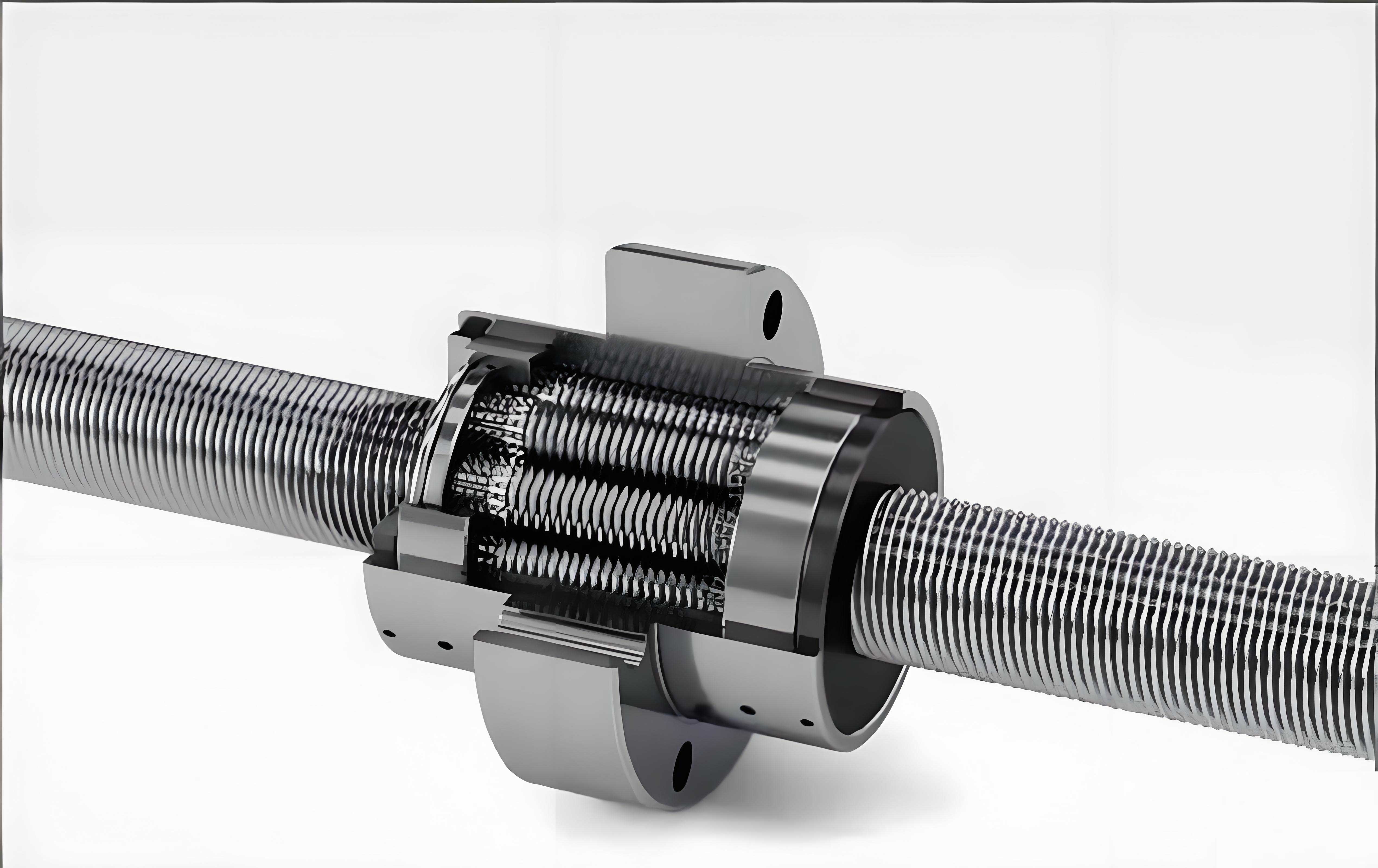
The rollers are distributed circumferentially by a cage and engage with an internal gear ring at their ends to maintain proper phasing. This multi-contact, multi-body interaction generates complex vibration signatures that are modulated by its kinematics and any incipient faults.
To overcome the limitations of classical methods, we employ Deep Support Vector Data Description (Deep SVDD). This method integrates the hypersphere minimization objective of SVDD with the powerful feature learning capability of deep neural networks. Instead of using a fixed kernel, a neural network $\phi(\mathbf{x}; \mathbf{W})$ parameterized by weights $\mathbf{W}$ is trained to learn an optimal mapping of the input data. The joint training objective is:
$$
\min_{\mathbf{W}} \quad \frac{1}{n} \sum_{i=1}^{n} \|\phi(\mathbf{x}_i; \mathbf{W}) – \mathbf{c}\|^2 + \frac{\lambda}{2} \sum_{l=1}^{L} \|\mathbf{W}^l\|_F^2
$$
The network is trained to map normal data points as close as possible to a pre-defined center $\mathbf{c}$ (often chosen as the mean of the initial network outputs), thereby implicitly defining the minimal hypersphere in the learned feature space. The $L_2$ regularization term prevents overfitting. The anomaly score for a new sample is its squared distance from the center in this learned space: $s(\mathbf{x}) = \|\phi(\mathbf{x}; \mathbf{W}) – \mathbf{c}\|^2$.
Proposed Methodology for Planetary Roller Screw Assembly Fault Detection
The complete workflow for fault detection in a planetary roller screw assembly using Deep SVDD consists of several key stages: data acquisition, signal processing and augmentation, feature extraction, model training, and evaluation.
1. Data Acquisition and Preprocessing
Vibration data is collected from a planetary roller screw assembly test rig under different health states. The test rig typically includes a servo motor, coupling, the unit under test (the PRSA), and a loading system (e.g., hydraulic). For validating a one-class approach, data is needed for at least two distinct states: a “Normal” healthy condition, and one or more “Fault” conditions. Common fault modes for a planetary roller screw assembly include lubrication failure, roller chipping or fracture, thread wear, and misalignment. In our experimental setup, tri-axial accelerometers are mounted on the nut housing to capture vibration signals. The signals are sampled at a sufficiently high frequency (e.g., 20 kHz) to capture relevant frequency components related to the meshing and structural dynamics of the planetary roller screw assembly.
Data Normalization: Raw vibration signals from different channels and runs are normalized to a common scale, typically $[-1, 1]$, to ensure stable and efficient neural network training. This preserves the directional nature of the acceleration data.
$$
x_{\text{norm}} = 2 \cdot \frac{x – \min(X)}{\max(X) – \min(X)} – 1
$$
Data Augmentation via Window Slicing: A major challenge in data-driven fault detection is the limited amount of available data, especially for fault conditions. To artificially enlarge the training dataset and improve model generalization, we employ a simple yet effective window slicing technique on the long time-series signals. A window of fixed length $W$ slides over the signal with a stride $S$, creating multiple shorter samples. The number of generated samples $P$ from a signal of length $N$ is:
$$
P = 1 + \left\lfloor \frac{N – W}{S} \right\rfloor
$$
This process is applied to all data channels, effectively increasing the number of training instances available for the model.
2. Feature Extraction via Wavelet Packet Transform
The vibration signals from a planetary roller screw assembly are non-stationary, often containing transient impulses indicative of faults. Time-frequency analysis methods are therefore superior to simple time-domain or frequency-domain analysis. The Wavelet Packet Transform (WPT) is employed for its ability to provide a fine, adaptive frequency resolution across the entire signal bandwidth.
WPT decomposes a signal into a complete binary tree of wavelet packet coefficients. At each decomposition level $j$, the signal is split into approximation coefficients (low-frequency band) and detail coefficients (high-frequency band) using quadrature mirror filters $h[k]$ (low-pass) and $g[k]$ (high-pass), derived from the chosen mother wavelet (e.g., Daubechies). The iterative decomposition formulas for the wavelet packet coefficients $W_{j+1, 2p}[n]$ and $W_{j+1, 2p+1}[n]$ at node $(j+1, p)$ are:
$$
W_{j+1, 2p}[n] = \sum_{k} h[k – 2n] W_{j, p}[k]
$$
$$
W_{j+1, 2p+1}[n] = \sum_{k} g[k – 2n] W_{j, p}[k]
$$
We perform WPT decomposition up to a specified level (e.g., level 4). The coefficients from the final level, which represent the signal’s energy distribution across multiple fine frequency sub-bands, are then rearranged into a 2D matrix (Height $\times$ Width) for each vibration channel (X, Y, Z). These matrices from the three channels are stacked depth-wise to form a 3-channel 2D input, analogous to a multi-channel image, which is fed into the convolutional neural network. This representation captures the joint time-frequency-spatial characteristics of the planetary roller screw assembly vibration.
3. Deep SVDD Network Architecture and Training
Convolutional Neural Networks (CNNs) are ideally suited for processing the 2D WPT coefficient matrices due to their ability to capture local patterns and translational invariance. The designed network for the planetary roller screw assembly fault detector is a compact yet effective CNN. The architecture is summarized in the table below.
| Layer Type | Parameters / Output Shape | Activation |
|---|---|---|
| Input | (H, W, 3) | – |
| Conv2D | 32 filters, (5×5), stride 3 | LeakyReLU (α=0.2) |
| Conv2D | 64 filters, (5×5), stride 3 | LeakyReLU (α=0.2) |
| Conv2D | 128 filters, (5×5), stride 3 | LeakyReLU (α=0.2) |
| Flatten | – | – |
| Dense (Fully Connected) | 256 units | Linear (No activation for Deep SVDD mapping) |
The network maps an input sample $\mathbf{x}_i$ to a 256-dimensional feature vector $\phi(\mathbf{x}_i; \mathbf{W})$. The center $\mathbf{c}$ is initialized as the mean of the network outputs for an initial forward pass on a batch of normal data and is fixed during training. The Adam optimizer with a learning rate of 0.001 is used to minimize the Deep SVDD loss (Eq. 2). The model is trained exclusively on data from the normal operating condition of the planetary roller screw assembly. The training process aims to shrink the “volume” of the normal data cluster in the learned feature space.
4. Model Evaluation and Comparison
To evaluate the trained Deep SVDD model, a separate test set is used containing both normal samples and samples from various fault conditions (e.g., lubrication failure, roller tooth breakage). Since the test set is imbalanced (more fault samples if multiple faults are tested), standard accuracy is not a reliable metric. The Area Under the Receiver Operating Characteristic Curve (AUROC) is used. The ROC curve plots the True Positive Rate (TPR) against the False Positive Rate (FPR) at various threshold settings on the anomaly score $s(\mathbf{x})$. A perfect detector achieves an AUROC of 1.0, while a random classifier scores 0.5.
The performance of Deep SVDD is compared against two traditional one-class baselines:
1. One-Class SVM (OCSVM): Uses the hypersphere or hyperplane formulation in a kernel space.
2. Kernel SVDD: The traditional kernel-based SVDD method.
For a fair comparison, the same WPT-processed input features are used for OCSVM and SVDD. The critical kernel parameter $\gamma$ for the RBF kernel is tuned over a wide range.
Experimental Analysis and Results
Following the described methodology, experiments were conducted. The planetary roller screw assembly test rig was operated under three conditions: Normal, Lubrication Failure, and Roller Tooth Fracture on one side. The dataset was processed, augmented, and transformed via WPT. The final dataset splits are shown below:
| Dataset | Condition | Number of Samples | Label (for evaluation) |
|---|---|---|---|
| Training Set | Normal | 601 | 0 (Normal) |
| Test Set | Normal | 80 | 0 (Normal) |
| Lubrication Failure | 80 | 1 (Anomaly) | |
| Roller Tooth Fracture | 80 | 1 (Anomaly) |
The Deep SVDD model was trained for 50 epochs. The OCSVM and SVDD models were trained with the RBF kernel across 50 different $\gamma$ values. The primary results are summarized in the following table, which highlights the optimal performance of each model on the test set.
| Model | Best Test AUROC | Corresponding Parameter (γ) | Remarks |
|---|---|---|---|
| Deep SVDD | 0.996 | – | Stable convergence over epochs. |
| OCSVM | 0.767 | 0.10266 | Performance highly sensitive to γ. |
| Kernel SVDD | ~0.500 | 0.27608 (example) | Failed to learn a meaningful boundary (AUROC ≈ random guessing). |
The results clearly demonstrate the superiority of the Deep SVDD approach for fault detection in the planetary roller screw assembly. The key findings are:
1. Superior Detection Performance: Deep SVDD achieved a near-perfect AUROC of 0.996, significantly outperforming OCSVM (0.767) and completely surpassing the failed Kernel SVDD model. This indicates its exceptional ability to differentiate between the complex vibration signatures of a normal and a faulty planetary roller screw assembly.
2. Robust and Stable Training: The AUROC of Deep SVDD increased smoothly and stabilized over training epochs, showing consistent learning. In contrast, the performance of OCSVM fluctuated drastically with changes in the $\gamma$ parameter, making it difficult to tune reliably without extensive validation data—which is precisely what is lacking in one-class scenarios.
3. Effective Feature Learning: The failure of kernel SVDD and the mediocre performance of OCSVM suggest that the raw WPT coefficients (or their simple kernel transformations) do not form a linearly separable cluster in some implicit space for this specific problem. The CNN within Deep SVDD successfully learns a non-linear transformation $\phi(\cdot)$ that maps the normal samples into a tight cluster in the 256-D feature space, effectively “unmixing” the normal and abnormal patterns that are entangled in the original input space.
4. Training Efficiency: While a single training run of Deep SVDD involves multiple forward/backward passes, its modern optimizer converges efficiently. The total time to train for 50 epochs was notably lower than the cumulative time required to train and evaluate OCSVM across 50 different $\gamma$ values to find the best one. This makes Deep SVDD a more practical choice.
The mathematical explanation lies in the flexibility of the learned mapping. The kernel methods rely on a fixed, pre-defined similarity measure $K(\mathbf{x}_i, \mathbf{x}_j)$. The neural network in Deep SVDD, however, learns a data-adaptive similarity metric through its weights $\mathbf{W}$, defined by the distance in its output space: $d(\mathbf{x}_i, \mathbf{x}_j) = \|\phi(\mathbf{x}_i; \mathbf{W}) – \phi(\mathbf{x}_j; \mathbf{W})\|$. For the planetary roller screw assembly vibration data, this learned metric is far more discriminative.
Discussion and Practical Implications
The successful application of Deep SVDD opens a promising path for the condition-based maintenance of systems employing a planetary roller screw assembly. The method’s requirement for only normal state data for training aligns perfectly with real-world constraints, where fault data collection is a significant hurdle.
Advantages:
1. No Fault Data Required: The model is built solely on healthy operation data, bypassing the need to simulate or collect rare fault conditions.
2. Detection of Novel Faults: Since it models normality, it can theoretically flag any significant deviation, including unforeseen fault types not present in any training library.
3. End-to-End Feature Learning: Eliminates the need for manual feature engineering; the CNN automatically discovers relevant patterns from the time-frequency representation.
4. Strong Performance: As demonstrated, it provides highly reliable fault detection compared to classical one-class methods.
Considerations and Future Work:
1. Representative Normal Data: The model’s definition of “normal” is entirely defined by the training data. This data must encompass all acceptable variations in operating conditions (e.g., different loads, speeds, temperatures). Otherwise, benign operational changes could be misclassified as faults (a high false positive rate).
2. Hyperparameter Selection: While Deep SVDD has fewer critical hyperparameters than kernel methods, choices related to network architecture (depth, width), the WPT decomposition level, and the preprocessing window size still need to be made, often via cross-validation on a held-out normal validation set.
3. Multi-Sensor Fusion: The current approach uses only vibration data. Integrating other sensor modalities like motor current, temperature, and acoustic emissions into the Deep SVDD framework (e.g., using multi-input networks) could provide a more robust health assessment of the planetary roller screw assembly.
4. From Detection to Diagnosis: While this method excels at answering “Is there a fault?”, the logical next step is to integrate it with auxiliary techniques (e.g., spectral analysis on flagged anomalies, or separate lightweight classifiers) to provide preliminary fault type identification, transitioning from fault detection towards fault diagnosis.
Conclusion
This work presents a comprehensive and effective framework for the fault detection of planetary roller screw assemblies using a one-class deep learning methodology. The proposed approach, centered on Deep Support Vector Data Description (Deep SVDD), directly addresses the practical challenge of limited fault data availability. By processing vibration signals through Wavelet Packet Transform and employing a Convolutional Neural Network to learn an optimal feature representation of normal operation, the method constructs a highly discriminative model of health. Experimental validation on a planetary roller screw assembly test rig, involving conditions such as lubrication failure and roller tooth fracture, demonstrated the model’s superior performance. It achieved an AUROC of 0.996, significantly outperforming traditional One-Class SVM and kernel SVDD, while also offering more stable training and greater practicality. The results affirm that Deep SVDD is a powerful and suitable tool for real-world health monitoring and incipient fault detection in critical mechanical transmission components like the planetary roller screw assembly, providing a crucial layer of protection and enabling proactive maintenance strategies.