
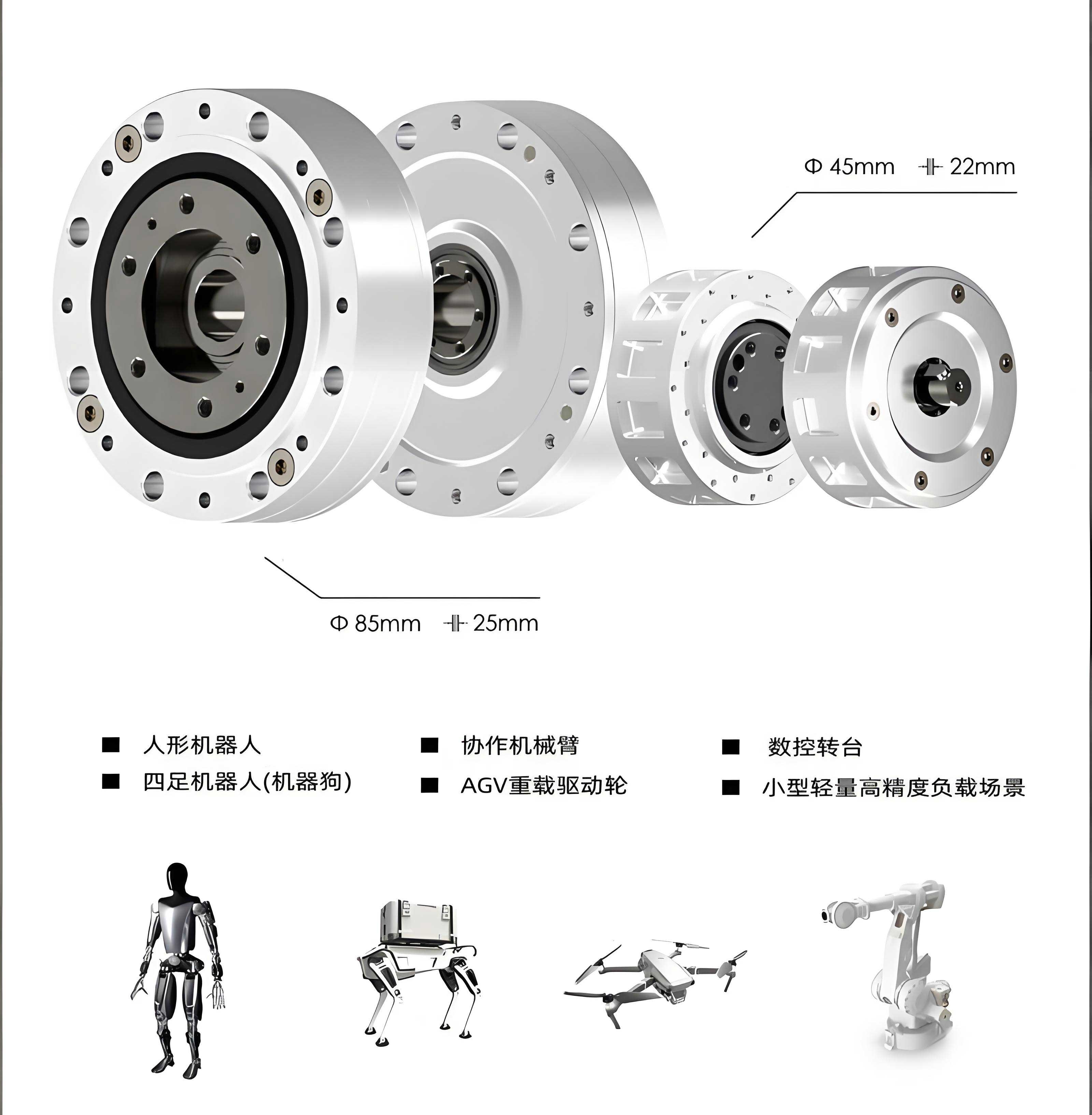
In the field of precision transmission systems, the RV reducer stands out as a critical component due to its high load capacity, compact design, and exceptional accuracy. As an engineer specializing in mechanical reliability, I have extensively studied the dynamic behavior of rolling bearings within RV reducers, as their performance directly impacts the overall system’s durability and efficiency. Rolling bearings in RV reducers operate under harsh conditions, including high loads and limited heat dissipation, making them prone to failure. Statistical data indicates that approximately 50% of mechanical failures in RV reducers are attributed to rolling bearing issues. Therefore, understanding the contact stress and deformation in these bearings is paramount for enhancing reliability. This article presents a comprehensive analysis using both Hertzian theory and finite element simulation, with a focus on the dynamic contact stress in RV reducer rolling bearings. I will detail the theoretical foundations, finite element modeling process, results comparison, and insights gained, aiming to provide a robust framework for optimizing RV reducer designs.
The RV reducer, derived from cycloidal pinwheel reducers, is widely used in robotics and aerospace applications. Its rolling bearings facilitate smooth motion transmission but are subjected to complex radial and axial loads. Traditional design approaches rely on Hertzian contact theory, which assumes small contact areas and linear elasticity. However, this theory has limitations in capturing real-world dynamics, such as friction and non-linear material behavior. In my research, I employ finite element analysis (FEA) via ANSYS Workbench to simulate the transient dynamics of rolling bearings in an RV reducer. This method allows for a more accurate assessment of stress distribution and deformation, enabling better design decisions. Throughout this article, I will emphasize the importance of the RV reducer in modern machinery and how advanced simulation techniques can mitigate failure risks. By integrating theoretical calculations with FEA, I demonstrate a practical approach to analyzing RV reducer rolling bearings, which can be extended to other high-precision transmission systems.
To begin, I review the Hertzian point contact theory, which forms the basis for calculating contact stress in rolling bearings. The Hertz theory applies to non-conforming contacts, where the contact area is small relative to the curvature radii of the bodies. For an RV reducer rolling bearing, the contact between rolling elements and raceways is typically modeled as a point contact, resulting in an elliptical contact area with a semi-ellipsoidal pressure distribution. The key assumptions include linear elasticity, smooth surfaces with no friction, and small contact dimensions. The fundamental formulas are derived as follows. The sum of principal curvatures is given by:
$$ \sum \rho = \rho_{11} + \rho_{12} + \rho_{21} + \rho_{22} $$
where $\rho_{ij}$ represents the principal curvatures of the contacting bodies. The difference function of principal curvatures is:
$$ E(\rho) = \frac{(\rho_{11} – \rho_{12}) + (\rho_{21} – \rho_{22})}{\sum \rho} $$
The semi-major axis \(a\) and semi-minor axis \(b\) of the contact ellipse are calculated as:
$$ a = n_a \cdot \left( \frac{3 \eta Q}{2 \sum \rho} \right)^{1/3} $$
$$ b = n_b \cdot \left( \frac{3 \eta Q}{2 \sum \rho} \right)^{1/3} $$
Here, \(Q\) is the normal contact load between the rolling element and raceway, \(\eta\) is a dimensionless parameter dependent on the material’s elastic modulus \(E\) and Poisson’s ratio \(\nu\), and \(n_a\), \(n_b\) are coefficients derived from Hertzian tables. The maximum contact stress \(\sigma_{\text{max}}\) is expressed as:
$$ \sigma_{\text{max}} = n_P \cdot \left( \frac{3Q}{2\pi^3 \eta^2 (\sum \rho)^2} \right)^{1/3} $$
where \(n_P\) is the peak stress coefficient. The contact deformation \(\delta\) is given by:
$$ \delta = n_{\delta} \cdot \left( \frac{9 \eta^2 Q^2}{32 \sum \rho} \right)^{1/3} $$
with \(n_{\delta}\) as the deformation coefficient. For an RV reducer rolling bearing under radial load, the normal load per rolling element is:
$$ Q = \frac{2F_r}{z \cos \alpha} = \frac{2F_r}{z} $$
assuming a contact angle \(\alpha = 0\) for simplicity, where \(F_r\) is the radial force and \(z\) is the number of rolling elements. In my analysis, I consider a specific RV reducer model, RV-40E, with bearing geometry: outer diameter 35 mm, inner diameter 15 mm, rolling element diameter 7.2 mm, width 10.8 mm, and 8 rolling elements. The material is GCr15 steel, with elastic modulus 207 GPa and Poisson’s ratio 0.3. The operational conditions for the RV reducer are summarized in the table below, detailing input speeds and torques across different scenarios.
| Scenario Type | Input Speed (rad/min) | Input Torque (N·m) |
|---|---|---|
| 1 | 405 | 7.06 |
| 2 | 810 | 5.74 |
| 3 | 1620 | 4.65 |
| 4 | 2025 | 4.358 |
| 5 | 2835 | 3.79 |
Using these parameters, I compute the theoretical contact stress and deformation for the RV reducer rolling bearing. The results are tabulated below, showing values for both inner and outer raceway contacts. These calculations serve as a benchmark for comparing with finite element simulations, highlighting the traditional approach to analyzing RV reducer components.
| Scenario Type | Inner Raceway Max Stress $\sigma_{1\text{max}}$ (MPa) | Inner Contact Deformation $\delta_1$ (mm) | Outer Raceway Max Stress $\sigma_{2\text{max}}$ (MPa) | Outer Contact Deformation $\delta_2$ (mm) |
|---|---|---|---|---|
| 1 | 5642.3 | 0.6378 | 5768.3 | 0.6543 |
| 2 | 4378.5 | 0.5623 | 4554.8 | 0.5828 |
| 3 | 3983.7 | 0.4732 | 4028.7 | 0.4926 |
| 4 | 3654.4 | 0.3928 | 3702.9 | 0.4095 |
| 5 | 2989.8 | 0.3254 | 3019.3 | 0.3667 |
Transitioning to finite element analysis, I employ ANSYS Workbench 15.0 to simulate the dynamic contact behavior of the RV reducer rolling bearing. FEA discretizes the continuous structure into finite elements connected by nodes, allowing for detailed stress and deformation analysis under complex loading conditions. This method overcomes the limitations of Hertzian theory by incorporating factors like friction and transient effects. For the RV reducer bearing, I create a 3D model using Pro/Engineer 5.0, simplifying it by omitting non-critical components such as the cage to reduce computational cost. The assembly includes inner and outer rings with rolling elements, and I model a quarter-section due to symmetry, which efficiently captures contact phenomena while conserving resources.
In the FEA preprocessing stage, I define material properties identical to the theoretical analysis: GCr15 steel with \(E = 207 \text{ GPa}\) and \(\nu = 0.3\). Mesh generation is crucial for accuracy; I use automatic meshing with refinement in contact regions. The contact zones between rolling elements and raceways are densely meshed to a size half of the contact ellipse’s minor axis, ensuring precise stress resolution. The mesh comprises 88,310 elements and 162,732 nodes, as illustrated in the model. Contact pairs are set with rolling element surfaces as contact faces and raceway surfaces as target faces, following best practices: convex surfaces contact planar or concave targets, and stiffer surfaces are designated as targets. I define friction contacts with a coefficient of 0.25, asymmetric contact behavior, and a normal stiffness factor of 0.8 to mimic real-world interactions in the RV reducer.
Boundary conditions and loads are applied to replicate the RV reducer’s operational environment. The outer ring is fully constrained on its circumferential surface to simulate bearing housing support, while the inner and outer ring sides have frictionless supports to restrict axial displacement. Rolling elements are constrained axially and tangentially, permitting only radial elastic deformation to prevent rigid body motion during transient analysis. Loads include inertial effects (gravity and rotational speed) and non-inertial radial forces. I apply gravitational acceleration globally, a rotational speed to the inner ring to induce motion, and radial bearing loads on the inner ring’s inner surface. These settings enable a realistic simulation of the RV reducer rolling bearing under dynamic conditions, capturing stress variations over time.
The transient dynamics analysis yields detailed stress and deformation contours for each operational scenario. For instance, at Scenario 1 (input speed 405 rad/min, torque 7.06 N·m), the maximum contact stress occurs at the contact points between rolling elements and raceways, with elliptical stress distributions radiating outward. The stress is highest at the center and diminishes towards the edges, consistent with Hertzian predictions. Similarly, deformation patterns show localized compression at contact areas. The results for all scenarios are summarized in the table below, providing a comparison with theoretical values. This FEA approach reveals nuanced stress distributions that are invaluable for optimizing the RV reducer’s bearing design, especially in high-load applications.
| Scenario Type | Inner Raceway Max Stress $\sigma_{1\text{max}}$ (MPa) | Inner Contact Deformation $\delta_1$ (mm) | Outer Raceway Max Stress $\sigma_{2\text{max}}$ (MPa) | Outer Contact Deformation $\delta_2$ (mm) |
|---|---|---|---|---|
| 1 | 5704.7 | 0.6556 | 5821.2 | 0.6689 |
| 2 | 4532.8 | 0.5834 | 4678.1 | 0.5947 |
| 3 | 4078.4 | 0.4954 | 4131.7 | 0.5017 |
| 4 | 3725.5 | 0.4014 | 3885.6 | 0.4281 |
| 5 | 3154.3 | 0.3473 | 3273.6 | 0.3725 |
Comparing the theoretical and FEA results, I observe a strong consistency, with relative errors within 10%. The error analysis can be visualized through curves plotting the discrepancies for inner and outer raceway contacts. For inner raceway stress and deformation, the relative error percentages are calculated as:
$$ \text{Error} = \frac{|\sigma_{\text{FEA}} – \sigma_{\text{Theory}}|}{\sigma_{\text{Theory}}} \times 100\% $$
These errors stem from several factors. First, FEA accounts for friction, whereas Hertzian theory assumes frictionless contact, making the simulation more representative of actual RV reducer conditions. Second, modeling simplifications and mesh discretization in FEA introduce minor inaccuracies. Despite this, the FEA results provide a comprehensive view of stress distribution, highlighting high-stress zones that require reinforcement in RV reducer bearings. The deformation trends also show non-linear behavior, with rapid changes in contact area under varying loads, which Hertzian theory cannot fully capture. This underscores the value of finite element analysis in enhancing the reliability of RV reducers through detailed dynamic assessment.
To further elucidate the findings, I discuss the implications for RV reducer design. The stress concentrations at contact points suggest potential fatigue initiation sites, which could lead to bearing failure in RV reducers over time. By using FEA, engineers can identify these critical areas and modify geometries or materials to mitigate risks. For example, optimizing the curvature of raceways or using advanced coatings can reduce peak stresses in RV reducer bearings. Additionally, the deformation analysis informs clearance and preload settings, ensuring smooth operation in RV reducers under diverse loads. The integration of FEA into the design process enables iterative improvements, reducing prototyping costs and accelerating development for high-performance RV reducers.
In terms of methodology, the finite element approach for RV reducer rolling bearings involves several best practices. Accurate modeling requires careful attention to contact definitions, mesh refinement, and boundary conditions. I recommend using symmetric models to reduce computational effort, as demonstrated in this study. Material non-linearities and thermal effects could be incorporated in future analyses to enhance realism for RV reducers operating in extreme environments. Moreover, validation with experimental data would strengthen the FEA predictions, providing a robust framework for certifying RV reducer components in industrial applications.
The advantages of FEA over traditional methods are manifold. It offers visual insights into stress and deformation patterns, facilitating intuitive design decisions for RV reducers. The ability to simulate transient dynamics allows for life prediction and reliability assessment, crucial for safety-critical systems like aerospace RV reducers. However, challenges remain, such as computational intensity and the need for expertise in setting up simulations. To address this, automated FEA tools tailored for RV reducer analyses could be developed, streamlining the process for engineers.
In conclusion, my analysis demonstrates the efficacy of combining Hertzian theory and finite element analysis to study dynamic contact stress in RV reducer rolling bearings. The theoretical calculations provide a baseline, while FEA delivers detailed, realistic insights into stress distribution and deformation. The results show good agreement, validating the FEA methodology for RV reducer applications. This approach enables optimized bearing design, enhancing the reliability and performance of RV reducers in demanding fields. Future work could explore multi-physics simulations, including thermal and wear effects, to further advance RV reducer technology. By leveraging advanced simulation techniques, we can push the boundaries of precision transmission systems, ensuring the continued evolution of RV reducers in modern machinery.
Reflecting on this study, I emphasize the importance of dynamic analysis in the context of RV reducers. As these components become integral to robotics and automation, understanding their mechanical behavior is key to innovation. The finite element method, as applied here, offers a powerful tool for probing complex contact phenomena, ultimately contributing to more durable and efficient RV reducers. I encourage researchers and engineers to adopt similar methodologies, fostering collaboration across disciplines to tackle the challenges in RV reducer design. Through continuous improvement, we can achieve higher standards of reliability and performance, solidifying the role of RV reducers in advanced mechanical systems.
To summarize the key equations used in this analysis for quick reference, I present them below in a consolidated form. These formulas are essential for both theoretical and computational studies of RV reducer rolling bearings.
Sum of principal curvatures:
$$ \sum \rho = \rho_{11} + \rho_{12} + \rho_{21} + \rho_{22} $$
Contact ellipse semi-axes:
$$ a = n_a \cdot \left( \frac{3 \eta Q}{2 \sum \rho} \right)^{1/3}, \quad b = n_b \cdot \left( \frac{3 \eta Q}{2 \sum \rho} \right)^{1/3} $$
Maximum contact stress:
$$ \sigma_{\text{max}} = n_P \cdot \left( \frac{3Q}{2\pi^3 \eta^2 (\sum \rho)^2} \right)^{1/3} $$
Contact deformation:
$$ \delta = n_{\delta} \cdot \left( \frac{9 \eta^2 Q^2}{32 \sum \rho} \right)^{1/3} $$
Normal load per rolling element:
$$ Q = \frac{2F_r}{z} $$
These equations, combined with finite element simulations, provide a comprehensive toolkit for analyzing and optimizing RV reducer rolling bearings. As technology advances, integrating machine learning with FEA could further enhance predictive capabilities, ushering in a new era of smart design for RV reducers and similar transmission systems.